OSDR Data Visualization Portal

The image displays the NASA logo, which is a red, white, and blue meatball design. Below the logo is the text "Open Science for Life in Space". To the right of the text is the website's navigation menu the "Data Visualization” is highlighted with blue text, surrounded by a red box and has an red arrow pointing at it.

• The OSDR has many data visualization tools suitable for multiple applications and stakeholders.

  • Data & Tools: Use the dropdown menu to access the “Data Visualization” hyperlink to open the OSDR multi-study data visualization application.

Metadata Dashboard

Link to Metadata Dashboard

The metadata dashboard is designed to help users narrow search results for experimental data. It provides various tools for filtering and displaying results.

• The main tools for filtering the study table’s results are the Pie charts and the filters on the left side of the dashboard. Each section of the Pie chart acts as a separate section of filters, and when a filter from the Pie chart is selected the results containing that factor will automatically populate in the studies table below. A user can make one selection on each Pi chart to narrow the results in the studies table. On the left side of the dashboard are a series of filtering options that can be used to identify similar studies. At the bottom of the page is a table summarizing the main metadata that describes how these studies were conducted.

  • At the bottom left of the table, there is a blue “Visualize Study” button that will launch any combination of studies that can be selected into a new tab in your browser for further analysis

Image showing the OSDR data visualisation home page. 4 pie chart are divided into multiple colored sections. The text in the center above the pie chart says 438 studies are currently selected. The pie charts summarize the OSDR metadata values for Factors, Assay technology type, Organism and tissue. Below the pie charts is a time providing more details and the capacity to select individual or multiple studies for further analysis. To the left of the screen is a series of filter options that allow the users drill down into the datasets and find related studies.

Selecting “processed studies” to find higher-order data.

• Users can select factors as filters on the Pie charts or the left side of the dashboard, both sections will be updated to show the selected filters and the studies table will be updated to show the relevant studies.

  • At the top of the filter panel on the left of the screen, you can see the “Show only studies with processed data tab”, selecting this option and then pressing the “Apply” filter button that excludes studies without processed data.

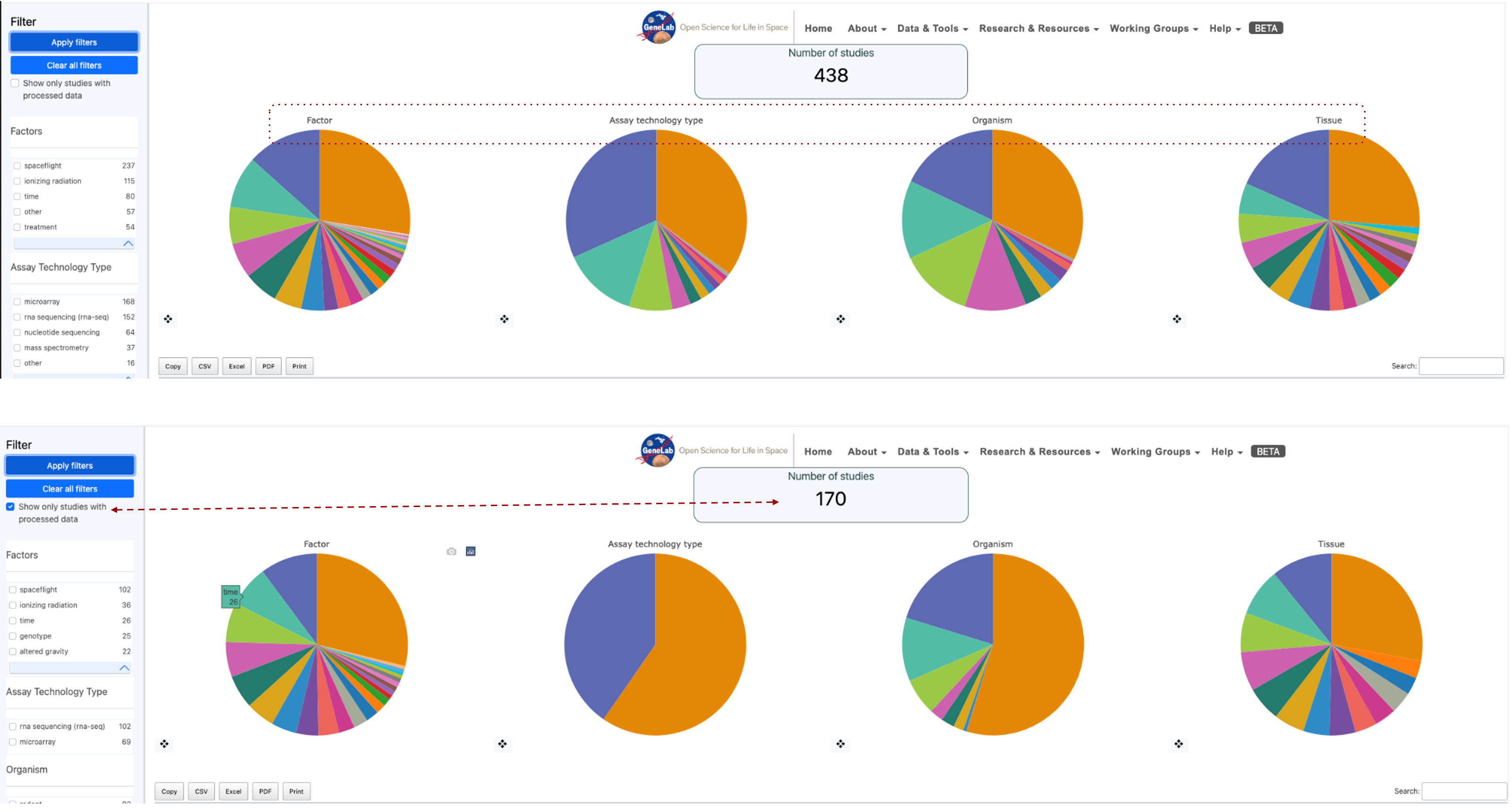
Image showing 2 screenshots of the metadata pie charts. The top row shows 438 studies and a red dotted box highlights the Factors, Assay technology types, Organism and Tissue titles on the pie charts to highlight they can be used as filters. The second row of pie charts is annotated with a red dashed arrow connecting the “Show only studies with processed data” option has been engaged and as a result the number of studies currently being selected has been reduced to 170.

Bar charts of factors

The bar graph displays the results per factor. When a factor is selected, it is broken down into types. After selecting a filter, the user can click “apply” to activate the filter and update the results on the graph. A red “X” appears next to the crosshair of the Pi chart to clear filters.

• Each pie chart comes with a crosshair tool located at the bottom left. Selecting the crosshair displays a bar graph showing the factors listed in the pie chart.

  • Example factors bar plot: In this example, the tissue factor has been viewed as a bar plot, and then the “Root” is selected, this then opens a new table that includes the 2 tissue ontology terms that contributed to the original “Root” ontology term. In this example “Root” is made up of both “plant root” and “root”

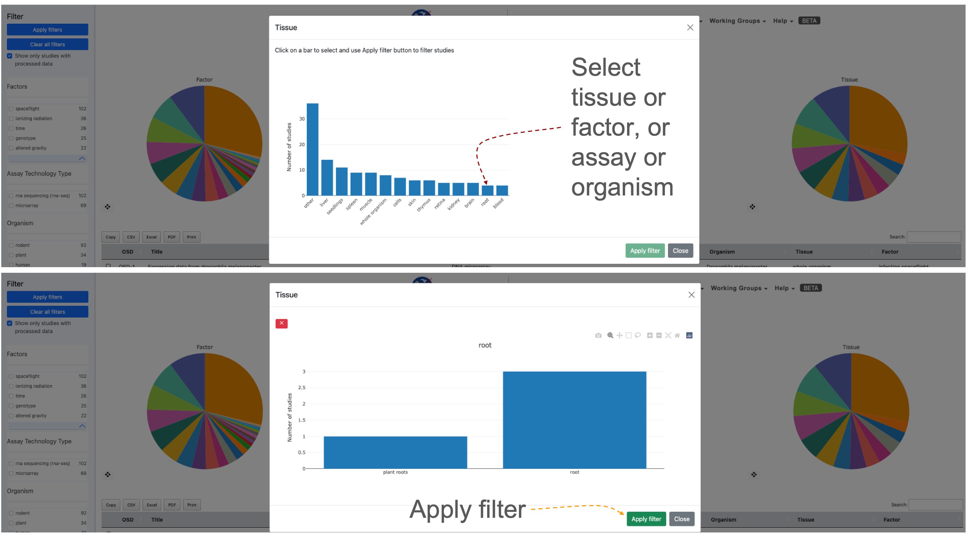
2 screenshots showing the “Tissue” metadata presented as bar charts. The red dashed line shows all the "tissue" options and highlights that in this example the “root” term is selected. In the bottom screenshot shows the 2 sub-terms that are combined in the “Root” term and an orange arrow pointing at the “Apply filter” button.

Selecting a study or group of studies for visualization

Once a user has selected a study or multiple studies they can press the “Visualize Study” button to be directed to the data visualization tools.

• You may also select multiple studies to visualize simultaneously in which case a user will be directed to a Multi-Study preview page before being directed to the data visualization tools.

  • Filtered down to one study example: A series of filters applied narrowed the selection to 1 study that fulfils all the user’s parameters. The red dashed lines highlight the box that allows the user to select a study, the screen image also shows how a selected study appears when it is highlighted and also identifies where the blue “Visualize Study” button can be found.

Image showing Four pie charts illustrate the metadata results determined by applying a series of filters to identify studies with similar organisms and tissues. Red arrows indicate where users can select studies of interest and highlight how the blue visualization study button can be utilized to activate the data visualization graphical user interface.

Studies Metadata Menu as a Table

At the bottom of the page below the pie charts is a table that lists the studies resulting from the selected filters from above.

• The table includes the following information for each study: OSD, Title, Assay, Organism, Tissue, and Factor. By default, the studies will be listed in order of OSD-# from smallest to largest, but the order can be reversed based on each information category by double-clicking on the study title.

  • First 10 in chronological order: If no list is applied then the table default is to show these in numerical order based on the OSD accession number.

Table showing the frist 8 OSD accessions providing their title, assay, organism, tissue, and factors being studied.

Selecting studies for Multi-study analysis:

The multi-study page is used to initialize the parameters for data visualization of the multiple studies. Researchers can uncover intricate patterns of gene expression associated with specific conditions or treatments across a variety of experiments. Below are detailed instructions on how to effectively navigate and utilize the Multi-Study Page.

• For your initial test, let’s use rodent studies as an example.

• Start by selecting “rodent” as the organism of interest. Since combining DNA microarray assays is not supported, ensure filtering by both “rodent” and “RNA sequencing” in the assay technology type.

• Choose two different rodent studies that encompass various tissue types. For instance, select “OSD-49” and “OSD-100.”

• Mark the checkboxes beside the selected studies in the studies table.

• Click the “Visualize Study” button to proceed.

• In this example OSD-49 & OSD100 have been selected, normalized with DESeq2 and their first 2 principle components plotted in a 2D scatter plot. To the right the is a factor selection tab where you can add new factors that will appear as columns beside the OSD-###. Clicking on the “Expand table” button reveals a table showing all the replicates and the metadata the user loads.

Screenshot showing the graphical user interface of the Multi-study visualization application showing data for OSD-49 & OSD-100.

Multi-study Data Normalization:

A dialogue box will appear to prompt you for data normalization options. The default selection is often “DESeq2” for normalization, but you can also choose “No Normalization.”

• E-mail notification: If desired, you can enter your email address to receive a notification when the studies have been combined and normalized. Alternatively, proceed without entering an email address.

• Normalization and PCA Insights: Understand normalization details by clicking the Information button next to the normalization method. View the PCA chart, which provides insights into data distribution after normalization.

• Factor Selection and Differential Gene Analysis: Under “Factor Selection,” choose variables to generate a factors table for differential gene analysis. Select parameters, characteristics, or factors from the dropdown list to add to the table.

• Exploring the Multi-Study Page: A PCA chart for data visualization will be included on the multi-study page. Utilize the PCA chart options to tailor your visualization based on specific criteria.

• Modifying Normalization Method: If you wish to change the normalization method (e.g., from “DESeq2” to “No Normalization”), click “Change Normalization Method.”

• Sample Selection for Gene Expression Analysis: Select specific samples by clicking the “Select labelled, expand table” button. Choose samples based on factors added during factor selection.

• Visualizing and Downloading Results: Click “Visualize Studies” to proceed to visualization plots or download the accounts table. Depending on your selection, enter your email address for a notification upon completion.

• Exploring Visualization Plots: Upon completion, the page will direct you to a range of visualization plots and graphs for your data analysis.

Multi-study Sidebar Functions

When a user has selected the study/studies to visualize, they will be directed to the data visualization tools, where a sidebar of helpful tools is provided on the left side of the screen.

The “Study Details” button is located at the top of the sidebar. This button pulls up a display with the study information including a small description. The display also includes a tab labelled “samples” that a user can press to see the individual samples and additional information for the study.

Below the study details button is a label for each plot provided for a user within the data visualization tool. Clicking these labels will automatically direct the user to the plot associated with the label.

At the bottom of the sidebar is the default Group selection is utilized for each plot. A user can modify the groups are selected by pressing the “Modify Groups” button. This button will prompt the user to select the individual groups that a user would like to see displayed on each plot.

A feature exclusive to multi-study visualization is the option to download the combined Differential Gene Expression (DGE) table.

Users can then select a threshold based on quantitative factors of gene expression such as fold change, P-value and Adjusted P-value.

When a user accesses the multi-study visualization the DGE table will have several options to export the information at the top of the table.

The sidebar allows users to go straight to specific types of data visualisation including PCA, Volcano, Scatter pairs, heatmaps, GSEA and tables of DESeq2 results.

Plotly

Plotly is a third-party software that uses data provided by OSDR to create the interactive visualizations displayed.

• At the top-right corner of each plot will be options to help a user better visualize the data. The house logo within the options will reset the axes of the plots back to default.

  • Users also have the option to zoom in/out on each plot as well as auto-scale the graphic. There are two tools provided for data point selection, the lasso tool and the box select tool. Each of these tools provides a shape that will select any data points that fall within them. Lastly, there is a download button in the shape of a camera that will let you download the plot as a PNG file.

Screenshot showing an example scatter plot made of red and blue dots. The % difference threshold is used to determine the relative proportions of red and bue. Above it is an enlarged version of the plotly panel of graph optimization options with the "Pan" button selected. The panel also has a button for copying a screenshot, minimising the screen, and maximising the screen, along with the lasso and square box selection tools.

PCA Plots

PCA stands for Principal Component Analysis, and this type of plot is used to reduce the dimensionality of large experiments to simplify the process of analyzing the data points.

Link to read about PCA plots

• Each PCA plot will include options for a 2D and 3D representation of the data. The default selection is a 3D representation on an “X”, “Y”, and “Z” axis. In the upper left corner of the plot area select the “2D” button and then press “Update” The graph will update to display the data on an “X”, and “Y” axis only.

  • The “Color by Factor” feature allows users to select a specific factor from the study for representation on the graph to allow for an easier comparison between differences in the data. Select the “Color by Factor” drop-down menu, within the drop-down menu select one factor, then press the “Update” button.

Screenshot showing the PCA plot results for GLDS-120. Replicates are presented as dots and their color defines a combination of their genotype and light treatment. The PCA plot is 3 dimensional but only the axis for PC1 and PC2 are shown. Above the graph are a series of options that can be used to enhance the graph such as transitioning to 2D or changing the color grouping option.

Selecting groups in PCA plots

PCR plots contain a lot of information, on some occasions selecting a fraction of the samples and plotting their PCA variations in 2D can often be a clear and simple method to highlight clustering.

• In this example, the “Cell Line” factor was selected from the drop-down. The results will now be represented by colors matching the factor selected. In this example, (OSD-154) the colors represent the different cell lines from the experiment and clearly show how the cell lines could be a factor in the differences between the data points.

  • Another feature within the PCA plot tool allows users to hide factors by selecting the label located on the right side of the plot. The two labels provided are the cell lines “GM15036” which is represented by blue, and “GM15510” represented by the color orange. Click on the label “GM15036” and the data points will be hidden as shown below. Click on the label “GM15036” a second time and the data will return to the graph.

2 PCA plots showing that users can toggle on and off different groups. Red dashed lines highlight where the name of the sample can be found on the figure legend and that if you click on it you can add or remove different samples and the rest of the plot will adjust.

Pair Plots

Link to read about Pair Plots

Pair plots are used for Exploratory Data Analysis, where the plot visualizes the data in order to find a relationship between variables that can be continuous or categorical.

• A “Pair Plot” is used to understand the best set of features to explain a relationship between two variables. It also helps to form simple classification models by making linear separations in a dataset.

  • Enhancing difference visualization: The default display for the pair plot will be the comparison between two sets of data with a % difference color threshold of 20%. Two plots will be displayed on the dashboard for the ability to compare multiple sets of data simultaneously. In this example on the right, we can see an increase in the threshold reduced the number loci annotated as red. Clicking each of the drop-down menus will allow a user to change which axis the sample data is displayed on.

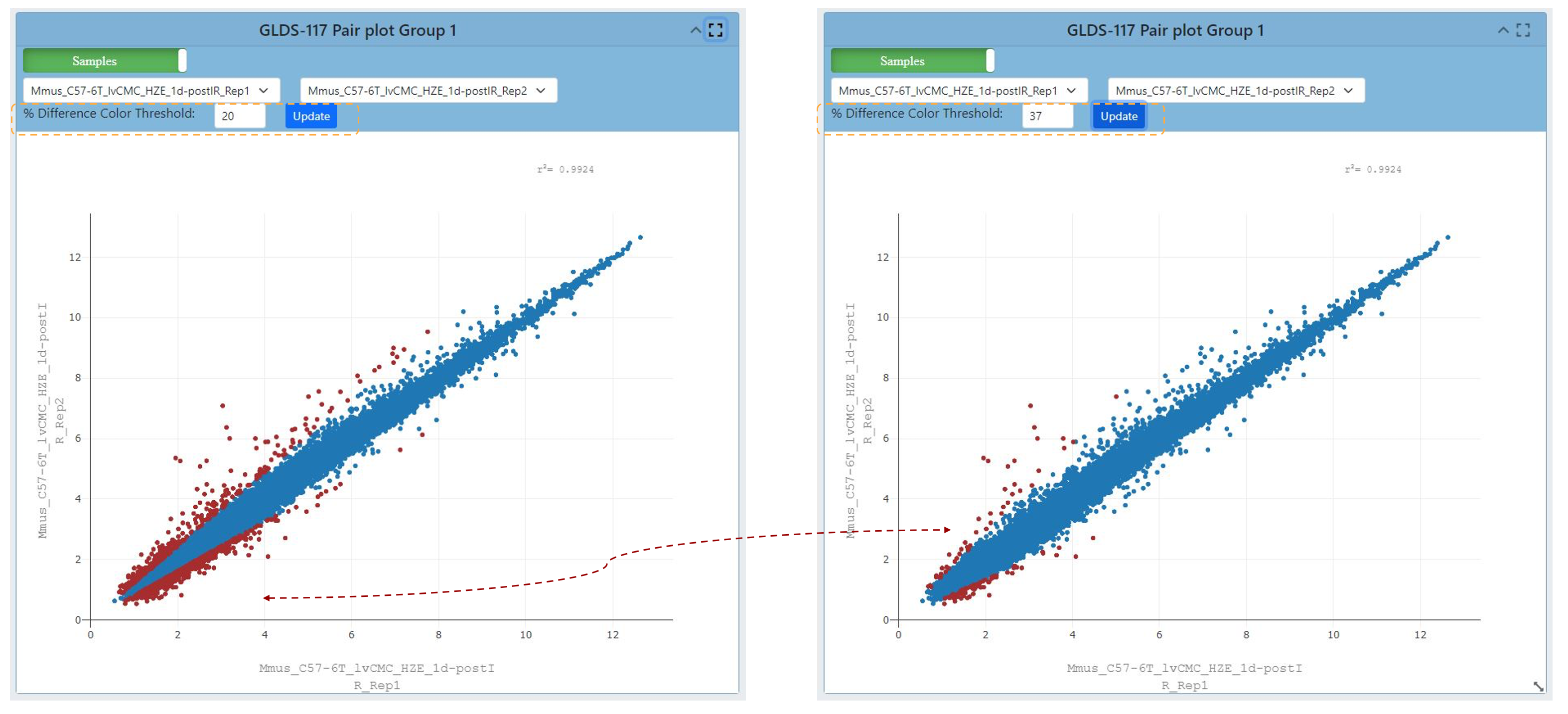
2 scatter plots, the graph on the right has had the % difference color threshold increase to 37. The red dashed line highlights the change in coloring caused by updating the graph after the threshold has been adjusted.

Refining Pair plot correlation visualization

Upon selecting the green “Samples” button located on the plot, one is presented with the opportunity to adjust several correlation coefficient values. These values serve to quantify both the strength and direction of the correlation that exists between data points.

• Coefficients closer to +1 indicate a strong positive correlation, while those near -1 suggest a strong negative correlation. A coefficient near 0 signifies a weak or no correlation. Selecting a different coefficient dynamically alters the spread of the data, with higher coefficients leading to tighter clustering and lower ones resulting in broader scattering.

• Users also can view different data correlations by clicking the green “Samples” button at the top of the plot and comparing it to other study providing a correlation coefficient summary. Clicking this button will change the dropdown to show multiple correlation coefficients for a pair of samples from the OSDR.

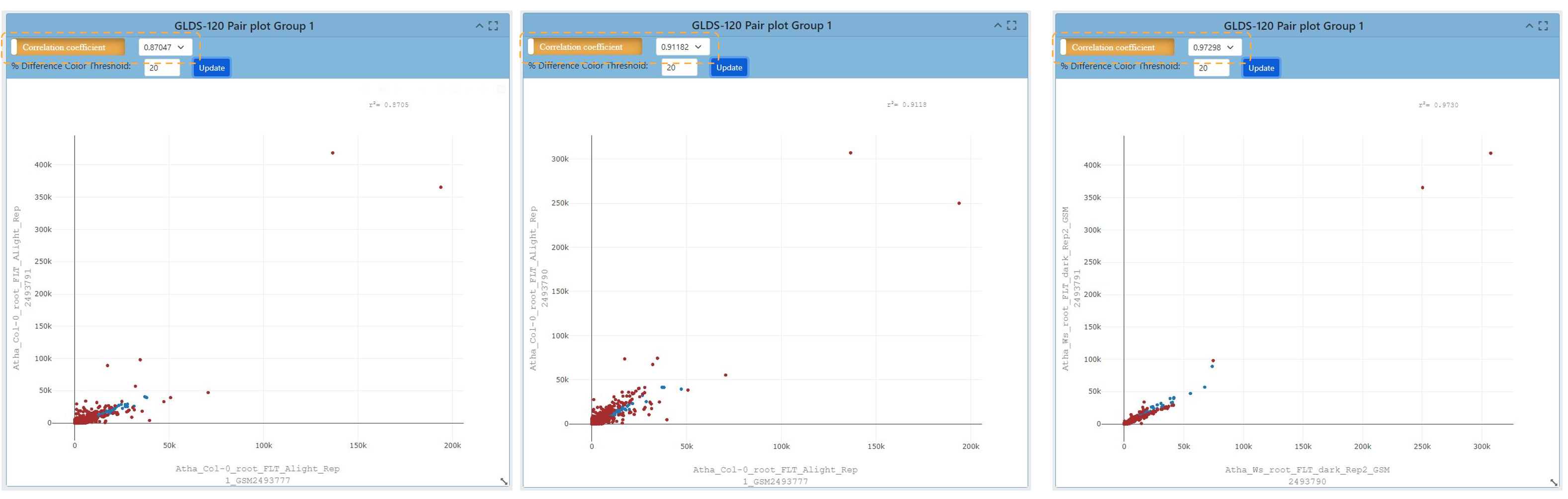
A screenshot presents four pairs of plots. The information presented in the plots comes from GLDS-120. Changing the correlation coefficient influences the number of samples and the spread of the data in the graph.

Volcano Plots

Link to read about Volcano Plots

The name volcano plot comes from its resemblance to a volcanic eruption with the most significant points at the top, like spewed pieces of molten lava.

• A volcano plot is useful for identifying events that differ significantly between two groups of experimental subjects. The default display for Volcano Plots will have the -Log10(Adj P Value) with an Adj P Value threshold of 0.05 and a Log2 FC threshold of 1.00 as shown below.

  • Each point on the graph represents a gene: The log2-fold differences between the groups are plotted on the x-axis and the -log10 p-value differences are plotted on the y-axis. The horizontal dashed line represents the significance threshold specified in the analysis, usually derived using a multiple testing correction.

Screenshot of a volcano plot presenting RNAseq data from OSD-120. Loci going up in abundance are red and loci going down in abundance are blue. A tab is highlighted allowing the user to change the values defined by the Y axis. The option -Log10(P-Value) is highlighted in blue and the results are presented on 2 adjacent volcano plots.

Customizing volcano plots

Adjusting the cutoff threshold for coloring the volcano plot and adjusting the distribution of data can increase the ease of data integration.

• Users can change the type of data displayed on the Y axis, and the options from the dropdown menu include “P Value, Adjusted P Value, and -Log10(P Value)”.

  • Below is an example of the “P-value”, adjusted P value and log10 (P-values) display for a volcano plot. In addition, the ability to change the P value threshold is available and the image below shows a P value and Log2 FC thresholds are also provided. In this example the threshold is increased to P values of 0.25 and a Log2 Fold Change threshold of 3 is applied.

Screenshot showing 4 different volcano plots demonstrating the effect of each of the different transformation options that can be plotted on the Y axis. To maintain the 'explosive' spread of data the -log10 transformation is essential and changing from adjusted P-values to just P-values increased the range of the data on the Y axis. The thresholds are highlighted with yellow boxes. The change the data distrubution caused by using P-values vs adjusted P-values is highlighted with a yellow circle and the effect of changing the Log2 Foldchange threshold is highlighted by yellow squares.

Heatmaps

Link to read about Heatmaps

Heatmaps allow researchers to quickly and easily identify patterns of gene expression that are associated with specific conditions or treatments and use color coding to indicate the magnitude of values.

• By measuring the number of RNA molecules produced by genes in a particular sample, researchers can determine the level of gene expression.

  • The default settings for the heat map are shown in the image below. The heatmap links genes depending on how alike they are based on the conditions set in the experiment.

  • Log2 Transformation: The Log2 transformation is available to enhance the display of genes with more pronounced differences. Applying Log2 transformation can reveal subtler variations in gene expression between conditions.

Screenshot a heatmap using data from OSD-120 using the default settings. An orange dashed box highlights the setting tab at the top of the screen. To left there is a figure legend showing the samples and the colors used to define them in the bar at the top heatmap X-axis. The text on the X axis is the names of the samples. To the right of the heatmap a dendrogram shows the connectivity of the sample’s gene expression. To the right of the dendrogram is a red to blue scale bar showing loci expression variation from 1 to 0.

Filtering Heatmaps

Users can filter the genes displayed on the heatmap based on their significance or fold change.

• Filtering by Significance (Adjusted p values) and log2 foldchange thresholds:

  • This filtering helps highlight genes with statistically significant expression changes. Analyze the heatmap to identify gene expression patterns associated with specific conditions or treatments.

  • Users can switch off the clustering of rows or columns of genes causing the dendrograms to be removed. This also affects how the heatmap links genes based on similarity. In some cases, toggling off these types of clustering can help focus on specific groups of genes and their expression patterns. Pay attention to color intensity and clustering.

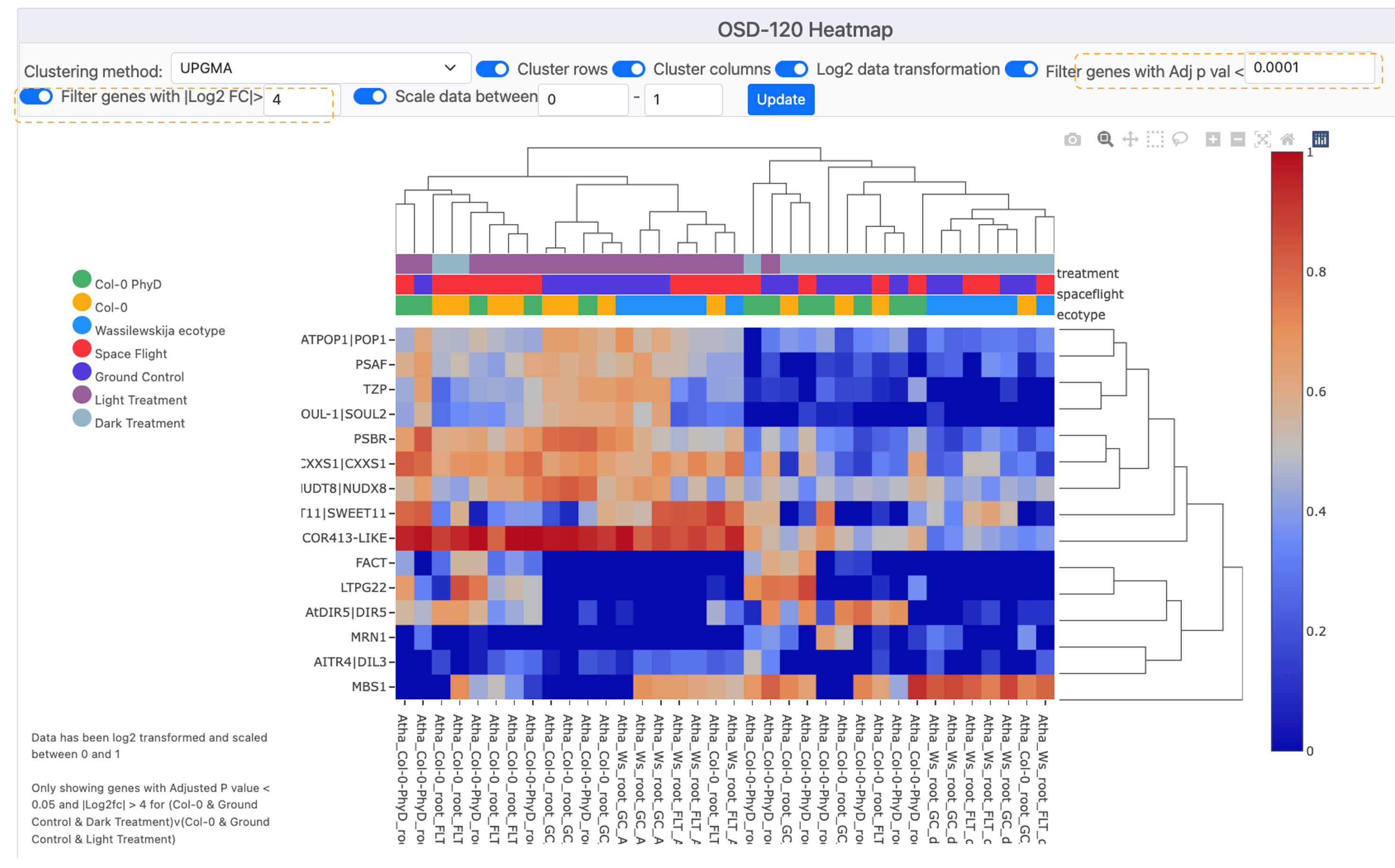
Screenshot showing a heatmap with fewer genes due to increasing the required log2F to >4 and also requiring a Adjusted P-vValue of less than <0.0001. These stringent criteria have reduced the number of loci displayed on the graph to 15 displaying the Symbol for each on the Y-axis. To left of the is a figure legend showing the colors used to define the sample metameta in the bar at the top heatmap X-axis. The text on the X axis is the names of the samples. To the right of the heat map a dendrogram shows the connectivity of the sample’s gene expression. To the right of the dendrogram is a red-to-blue scale bar showing loci expression change from 1 to 0.

Heat map clustering options

Users can select a clustering method to display results.

• Choosing Clustering Method: The default is often set to UPGMA (Unweighted Pair Group Method with Arithmetic Mean). Clustering helps group genes with similar expression profiles, making patterns more apparent so it can be useful to compare multiple options.

  • In this example we compare UPGMA to the Nearest Point Algorithm, Furthest Point Algorithm and the Ward variance minimization

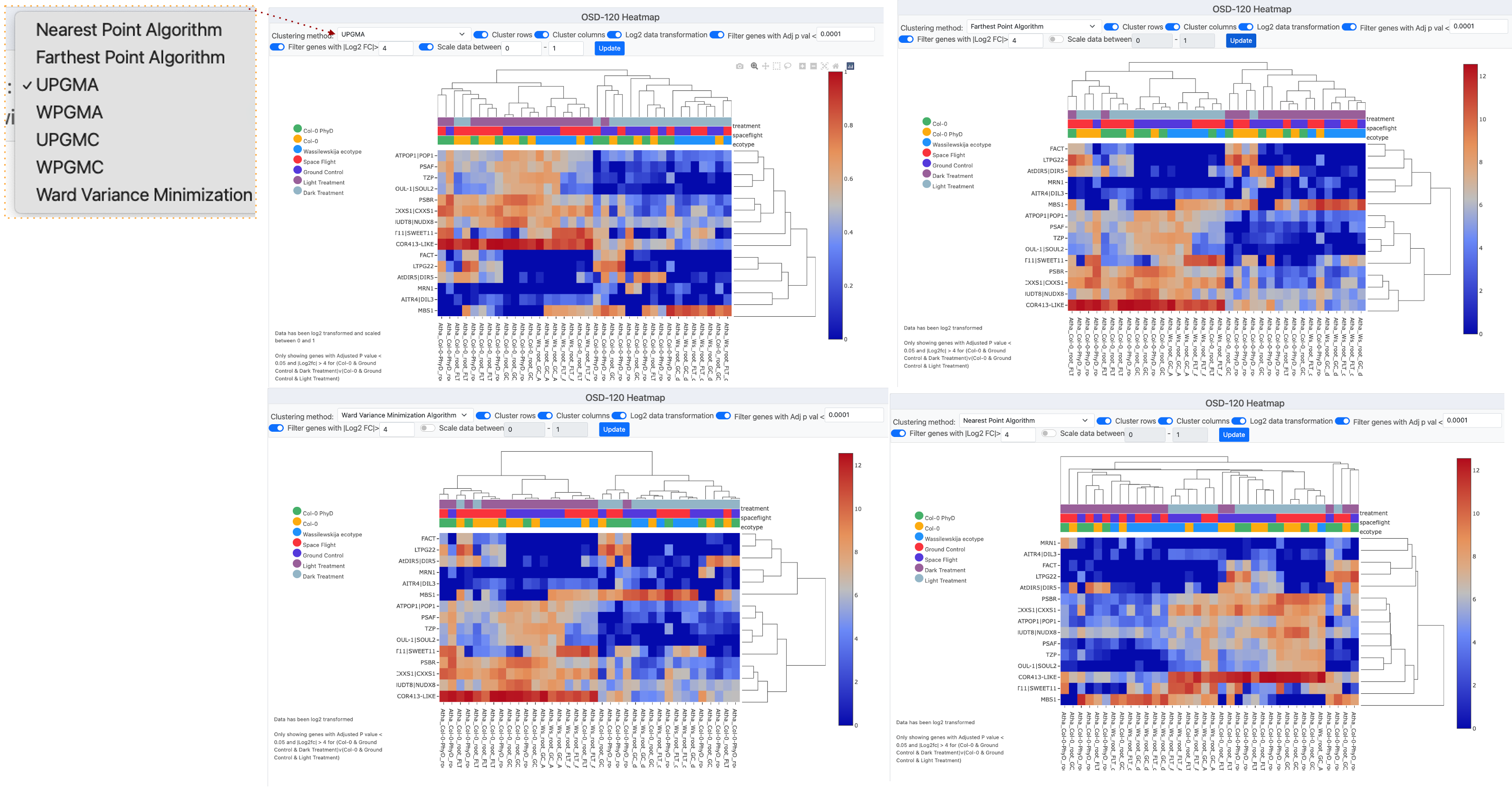
Screenshot montage showing 4 different clustering methods used to process the example data from OSD-120. In the left corner, there is a pop-up window that shows the “Clustering methods” menu which has been opened and the UPGMA method is currently selected.

Ideogram

Ideograms provide a schematic representation of chromosomes, and they are used to show the relative size of the chromosomes and their characteristic banding patterns.

Link to read about Ideograms

• The ideogram available through OSDR offers three options for customization.

  • Two options are related to how the user would like to filter significant genes, the first choice being genes with an adjusted P value less than the value set in the text box, and the second choice would be filtered by a Log2 FC value greater than the value set in the text box. The third option to customize the plot allows the user to change the layout of annotations for the Ideogram from a drop-down menu.

Screenshot showing 4 different types of Ideogram created using data from OSD-120. Each of the grey bars represents a chromosome and red lines or arroves depict where genes that are significantly differentially expressed genes can be found.

DGE Table

Each study will have an associated Differential Gene Expression (DGE) table available that includes information on each sample from the study.

To export a Differential Gene Expression (DGE) table from the study visualization page, follow these steps:

1. Locate the DGE Table: Scroll down to the bottom of the study visualization page. There, you’ll find the Differential Gene Expression table containing valuable data.

2. Copy the Table to Clipboard: Identify the “Copy” button within the DGE table. It should be prominently displayed. Click the “Copy” button. This action will copy the entire table, including all data, headers, and values, to your device’s clipboard which can then be placed into Word documents and/or spreadsheets.

3. Or save and export: As CSV, Excel, PDF, or send to Printer for a physical copy:

• To save the data in various file formats, look for the corresponding buttons.

  • For a CSV file: Locate and click the “CSV” button. This will prompt a download of the DGE table data in CSV format to your device.

  • For an Excel file: Look for the “Excel” button. Click it to initiate the download of the DGE table data in Excel format (XLSX) to your device.

  • For a PDF file: Find and select the “PDF” button. This action will convert the DGE table into a PDF file that you can save to your device.

  • For Printing: Spot the “Print” button. Clicking this will open a new window displaying a printer-friendly version of the DGE table. You can then use your browser’s print functionality to print the table directly.

Note: Choose the method that best suits your needs to access and analyze the DGE data efficiently.

Table showing 10 significantly differentially expressed mouse loci in the OSD-4. The table shows the Ensemble ID, Symbol, Log2FC, P-value and adjusted P-value. There are button in the top right hand corner that allow the user to down load these data.

Multiple study GSEA

GSEA stands for gene set enrichment analysis, a method to identify gene groups that are overrepresented in a large gene set. It uses statistics to pinpoint significantly enriched or depleted gene classes.

Link to read about GSEA

On the Gene Lab Visualization Portal, you’ll find a dedicated GSEA section for each study. Within this GSEA section, there are various parameters you can customize:

1. Choose genesets: Select the database geneset enrichment analysis. The default is “KEGG 2019,” which is recommended.

2. Permutations: Decide the number of permutations you desire and whether they’re based on phenotypes or gene sets.

3. Gene Number Range: Adjust the minimum and maximum gene sizes. Increasing the minimum size omits genes with fewer than 15 data points, same for the maximum size.

4. Weighted Score Type: Defaults to one, representing the t-test. Alternatively, choose signal-to-noise, fold change, or log2 fold change.

5. Statistical Method: Select your preferred statistical method. The default is the t-test.

To update the plot with your changes, simply click “Update.” A range of plot types is available:

• Normalized Enrichment Score (NES) Table: View different gene sets in a table format. Export this table using the options at the top.

• NES Plot: The default plot displays normalized enrichment scores based on gene sets.

• Dot Plot: Similar to NES Plot, it showcases the top six gene sets based on false discovery rate (FDR). FDR indicates the likelihood that a result is valid, e.g., FDR of 0.25 means a 25% chance of validity.

• Enrichment Plot: This reveals the fold change distribution of the top three gene sets with an FDR of under 0.25.

• Network Plot: Visualize relationships between gene sets using a network plot.

• GSEA Info: For in-depth details about GSEA creation, statistics, and plot documentation.

With these steps, you can effectively navigate and utilize the GSEA section, gaining insights into gene set enrichment analysis for your study. A more detailed explanation can be found in the earlier section on the OSDR single study data visualization application.