Navigating a single OSDR study

Identified a study of interest in the OSDR, after assessing the title, study descriptions and any related research paper you can use the data visualization application to learn more about some of the quantitative patterns within the data.

Single study: Navigate to a study of interest by searching through the study metadata you can launch the visualization menu using the visualization tab on the left menu.

Screenshot showing an example study from the OSDR.

Navigation panel

To the left of the screen is the navigation panel, this allows users to assess all the different sections of the repository and then go directly to the information they are looking for.

The navigation panel on the left a;llows you to move to sections of interst.

Study Overview: Title, icon, GeneLab ID, ALDSA ID and DOI

The top of the page contains the title of the study, the unique GeneLab ID, and if applicable, an ALSDA ID for other non-omics data such as photography or microscopy. The DOI provides a unique identifier for the entire study.

Description: Factors, organism, assay(s), project and contact information.

This section provides a description of the experiment, a summary of the factors, organism used, assays performed and project information.

Screenshot showing the project description infcluding the factors, organism, assay(s), project and contact information.

Experiments

Some studies provide descriptions of experiments, while others use the primary publication for this purpose. The OSDR now encourages all users to add a description of their experiment in the “Experiments” field.

Payloads

Flight mission(s) are sent to space flight environments as payloads on vehicles. These payloads are reif given operation identifiers to assist with flight operations.

In this example the payload identifier is CARA, this comes from its mission name “Characterizing Arabidopsis Root Attractions (CARA)”, along with a description of the experiment.

Missions

Experimental payload(s) are loaded in specific space flight “Missions”, these determine the launch vehicle, launch date and “end date”.

In this example, SpaceX-3 was the launch vehicle and the dragon then facilitated transit to the ISS and then back to Earth.

Protocols

The protocol section contains all the information related to how the samples were processed. This information variest depending on the study, but can include basic image acquisition protocols used by astronauts to more complex multi-stage sample processing and automated analysis that occurs with popular technology such as RNAseq.

Screenshot showing the protocol section, this study contains example photography acquisition and analysis descriptions.

Screenshot showing the protocol section, this study contains examples of nucleic acid extraction and library construction for RNAseq analysis.

Samples

Each experiment includes a sample(s) table detailing metadata about the experimental replicates. Information provided includes species, tissue type, genetic background, age at experiment completion, and treatment group (e.g., Flight or Ground). The bottom right-hand corner displays the total number of samples and the number currently being shown.

Screenshot with highlighted samples data and a organe dotted arroce highlight the "select export columns" button

Downloading sample metadata tables for further analysis

Clicking on the “Select export columns” button open a menu that allows users toggle on or off any of the samples metadata fields and can then choose to down the data as a table. This give the users the choice to select the factors they believe are important or download them.

Screen shot showing the samples data

Assays

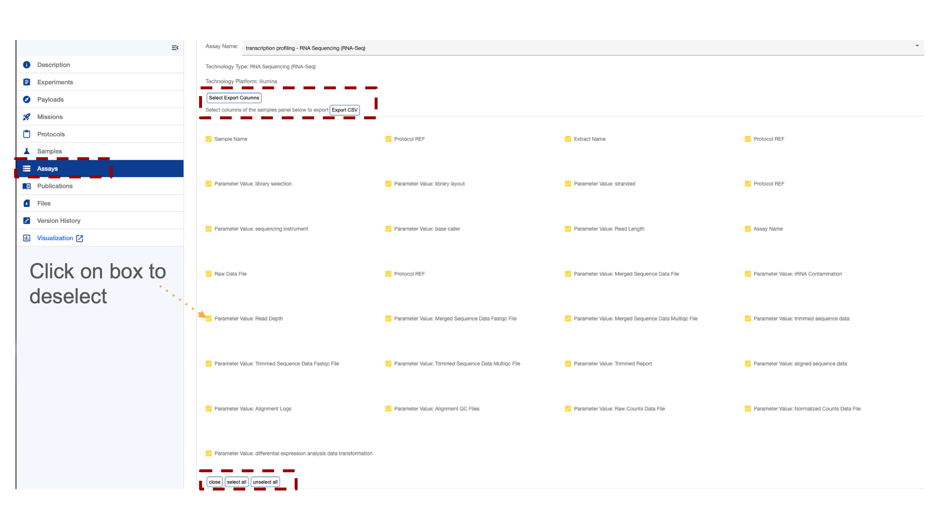
Several studies contain multiple assays which can be viewed separately. At the top right corner of the assay section, a toggle switch allows users to switch between assays. A scroll bar at the bottom of the screen facilitates navigation across the assay table. Many table entries are data products available for direct download and further inspection. There is a “select export columns” that opens the download menu.

Downloading assay metadata tables for further analysis

Clicking on the “Select export columns” button open a menu that allows users toggle on or off any of the assay metadata fields and can then choose to down the data as a table. This give the users the choice to select the factors they believe are important or download them.

Publications

The publication section includes links to related papers in the OSD repository, along with their titles, author lists, PubMed IDs, and DOIs.

Link to papers associated with the repostroy that is selected

Files

Files Section Overview

Access raw, intermediate, and high-order data products generated by the OSDR and GeneLab systems. Download data for further analysis by exploring the directory and clicking on the desired boxes.

Screenshot showing the folders of data in the repostory.

Screenshot showing the RNAseq subdirectory and some of the higher order data products that are avaliable.

Version History

The OSDR keeps a record of all previous analysis, users are advised to record the data Version they use and record it in any related metanalysis publications.

Visualisation

Most RNAseq and microarray data processed by the OSDR team can be viewed via the data visualization portal, accessible from the navigation on the studies repository page.

Single Study Visualization Navigation bar

The OSDR Visualization Navigation bar can allow you to navigate to a graph of interest.

• After launching the OSDR visualization application on the lefthand side of the screen you’ll see a navigation window that will allow you to select to go to the “Home,” “PCA,” “Volcano,”, “Pair plots”, “Heat maps”, “DGE”, “GSEA”, and Group Selection.

  • Single study navigation example: In this example, we see Group 1 of Col-0&FLT ( FLT is the flight group) and Group 2 is Col-0&GC (GC is the ground control group). https://visualization.genelab.nasa.gov/data/OSD-37

  • If a study has processed transcriptional data available then you can view it by launching it from the OSDR accession’s ”Visualization” button or by replacing the * wildcards in this website URL (https://visualization.genelab.nasa.gov/data/OSD-***) with the accession number of interest.

  • Clicking on these visualisation names allows the user to jump straight to the visualization of most interest.

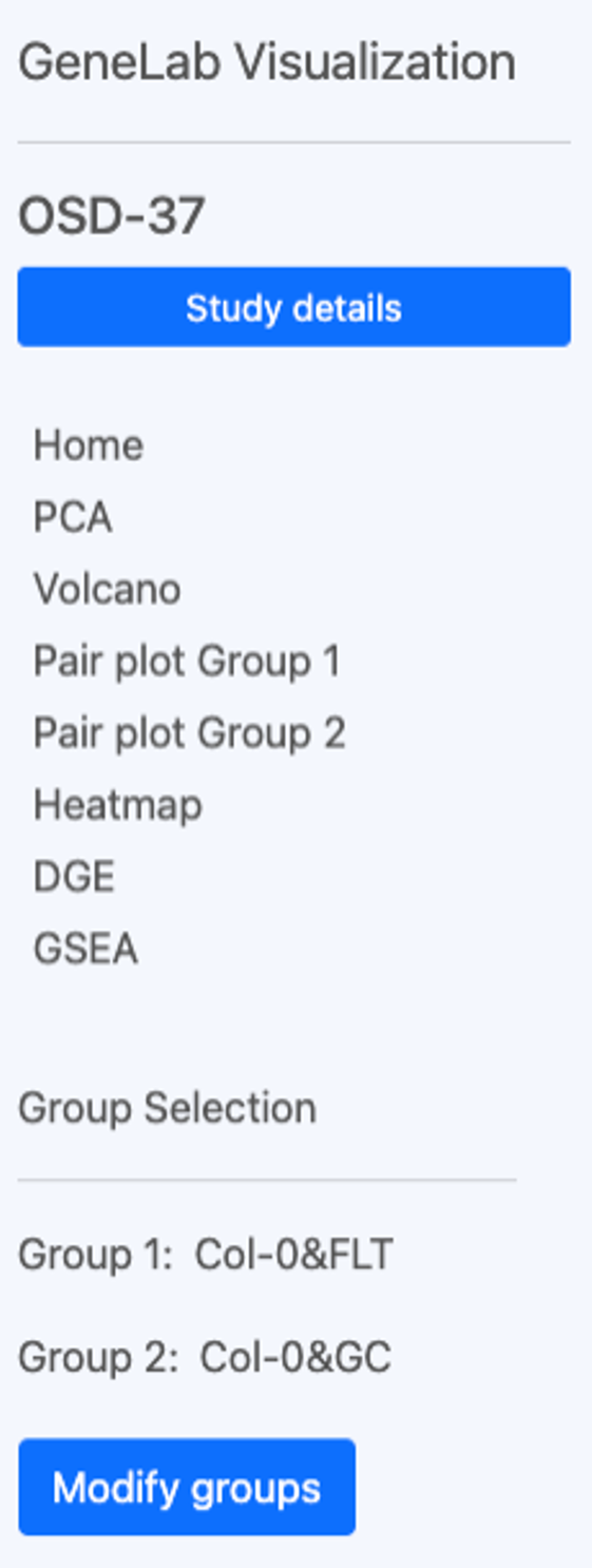
The OSDR Visualization interface includes the text "GeneLab Visualization" and "OSD-37," and a “Study details” search bar. Below is a verticle navigation menu with various options like "Home," "PCA," "Volcano,", “Pair plots”, “Heat maps”, “DGE”, “GSEA”, and “Group Selection”. In this example, it shows that Group 1 of Col-0&FLT (which is the flight group) and Group 2 is Col-0&GC (which is the ground control group). There is a “Modify groups” button in the bottom left corner that can be used to change the groups of samples used to generate the data in the plots

For more information go to the multi-study data visualization page.

Select Group(s)

Select Groups can be compared statically using the GeneLab data visualisation application.

• Space Flight (FLT) vs Ground control (GC) is a linear model often used to understand and identify genes, proteins and other omics data types that change in response to spaceflight (or related stimuli)

  • Single study grouping example: Select the sample group 1 and group 2 for differential comparison. You can deselect these groups by clicking on the blue check box or select them by clicking on the empty boxes. In this example, the user can compare the ecotype and treatment groups.

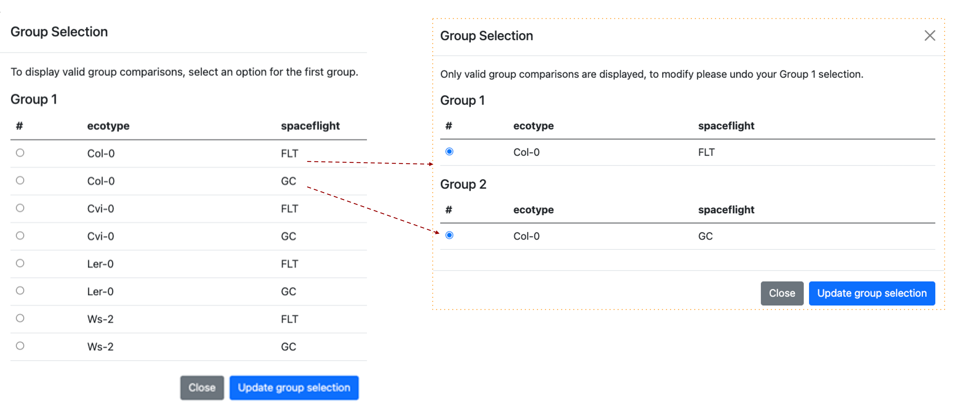
The images show the Group Selection screen. The screen is divided into two sections, each labelled with a group name and containing descriptions of the selected factors. In this example, it shows the "Ecotypes” and "treatments". A red dashed line highlights that when 2 groups are assigned a pop-up window shows the groups that are being compared.

Principal component analysis

Principal component analysis (PCA) shows clusters of samples based on their similarity.

• PCA: Click on samples to the right to select the desired samples to be viewed on the PCA plot. Icons on the upper right region of the plot allow for downloading, navigating and saving the plot. You can choose either 2D or 3D plots. If you click on the 3D graph and hold the left mouse button you can rotate the graph in 3D to optimise the angle and potentially highlight specific clustering patterns.

  • Single study PCA example: 3D plot has been selected and PC1, PC2, and PC3 are presented on the graph. Drop-down options allow users to replace these PC’s by selecting an alternative from the menu.

  • We can also see next to the “Color by factor” label that the current “all” is selected and the yellow arrow shows how the names of the factors have been combined in the figure legend.

  • It can be important to explore the PC’s that separate the data based on different factors as the main factor such as spaceflight might not always be captured by the first or second PC’s values. Sometimes results presented as a series of 2D PCA plots can be clearer than a 3D plot present 3 PC values.

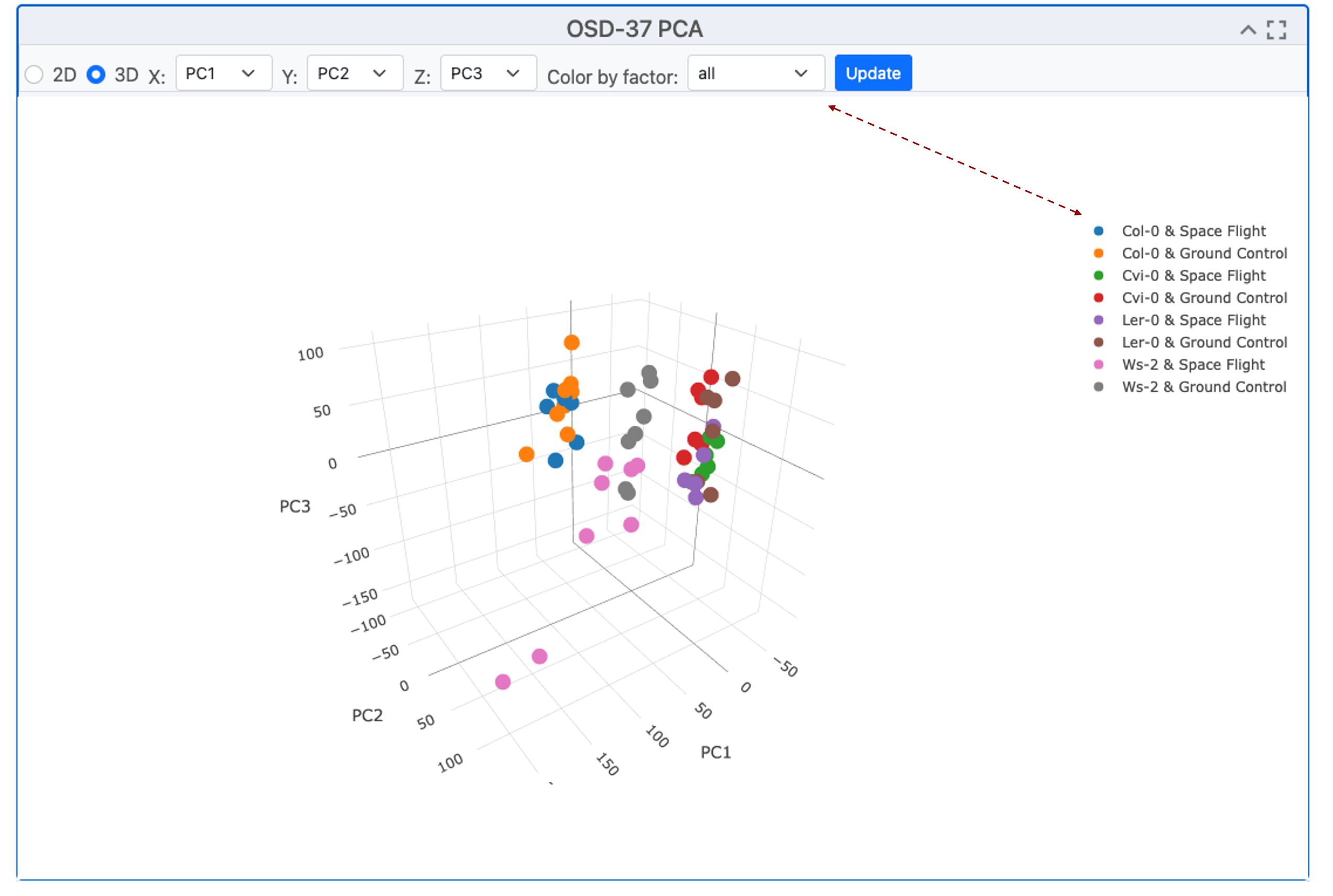
The scatter plot exemplifies the clustering of samples via Principal Component Analysis (PCA), a method that transforms correlated variables into uncorrelated ones called principal components. The plot presents the projection of samples onto the first two or 3 principal components, showcasing the majority of the variance in the original data. The clustering suggests the presence of distinct groups, indicating different characteristics captured by the principal components.

Pair plots

The “Pair plots” can be used to compare 2 samples from group 1 or group 2 respectively.

• Drop-down menus allow the researcher to select different replicates and view the comparative gene expression dispersion plots. This is useful for finding outlining samples or loci and the difference between each sample can be refined by adjusting the color threshold (default 20). In the top right-hand corner, there is a menu of graph-specific options, including snapshot, zoom, lasso, and full screen. The “update” button is highlighted in blue and needs to be pressed if you change any of the factors.

  • Pair plot replicate comparison example: We can see the % difference threshold is set to 20, we can also see the names of the samples being paired against one another and they are replicated of the same treatment.

Pair plots comparing 2 samples from Atha_Col-0_s1-pool_FLT_Rep4_R1-FL-B4 on the X axis and with Atha_Col-0_s1-pool_FLT_Rep4_R1-FL-B4 on the Y-axis. Loci are represented by red and blue dots. In the top right-hand corner, there is a menu of options, including snapshot, zoom, lasso, full screen, and the “update” button is highlighted in blue.

Volcano Plots

Volcano plots show statistical significance vs magnitude of change.

• To present the Volcano plot, the p-value is converted using a -log10 transformation to enhance the visibility of significant loci. The Fold Change (FC) is transformed using a Log2 transformation to balance the representation of upregulated and downregulated genes. This facilitates the identification of genes with significant statistical differences and substantial expression changes. Users can select parameters, samples for comparison, and the maximum adjusted p-value using the drop-down menu. The Log2 FC threshold can be adjusted using the menu bar at the top. The image can be exported or explored using the Zoom or Lasso tool to investigate specific clusters or outliers.

  • Volcano plot example: This graph generated by OSD-37 shows the adjusted P-value on the y-axis after it has experienced a -log10 transformation compared to the Log10 fold change (FC). In this example, SCPL50 appears to have a dramatic suppression during flight.

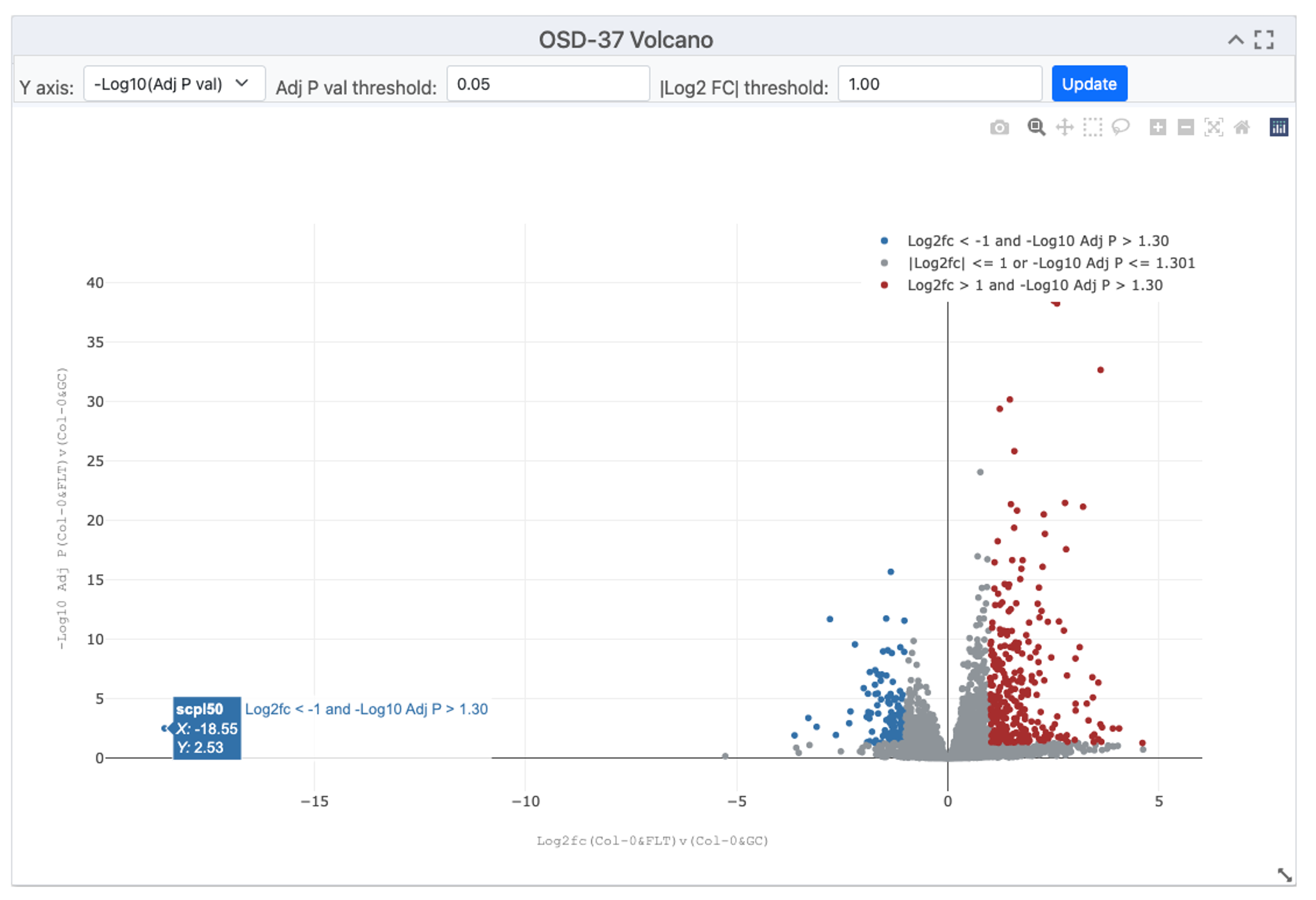
Image showing a volcano plot, with red dots representing genes with a significant increase in expression in orbit and blue dots representing genes that expression that was potentially suppressed by spaceflight-related factors. Drop-down menu allows for the selection of parameters, samples for comparison and maximum adjusted p-value. Some tabs also enable the transformation of the Y axis, the threshold of the adjusted P-value and the threshold of the Log2 FC can be adjusted using the menu bar at the top.

Table of gene expression data

A summary table of data compiling gene RefSeq IDs, Symbols, Log2Fc, P values, and Adjusted-P-values is often the most concise way to view data.

• In the top right-hand corner, boxes allow the user to filter the table based on the maximum P-VAL (P-value), maximum ADJP (adjusted P-value), LOG2FC (Log2 transformed fold change) or to just search for gene REFSEQ ID or gene Symbol (Name). In the top left of the table, the buttons allow the user to copy, export to CVS, Excel, PDF or even directly Print.

  • Summary of results example: This table shows the top 10 most significantly differentially expressed loci from OSD-37. The maxim adjusted p-value is set to 0.05, in the bottom left it shows 2445 entries selected by this threshold, in the bottom right it shows that there are 245 pages of data (as the screen had been adjusted to show 10 loci per page). These can be downloaded for further analysis.

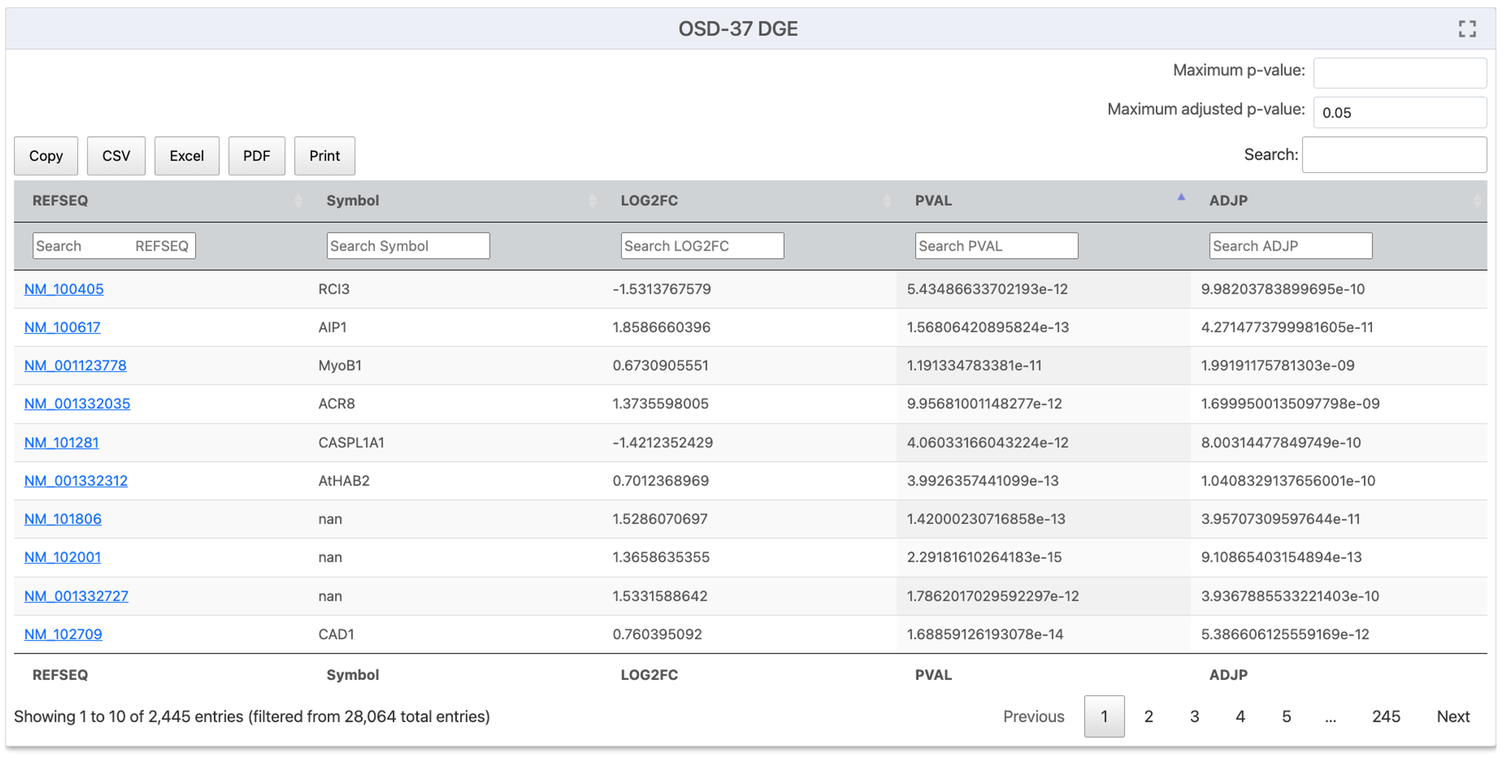
A screenshot from OSDR data visualization titled "OSD-37 DGE" showing a list of Gene REFSEQ IDs and Gene Symbols, along with their LOG2FC, PVAL and ADJP values. In the top right corner, there are boxes where users can enter values for P-VAL (P-value), maximum ADJP (adjusted P-value), LOG2FC (Log2 transformed fold change) or just search for particular gene REFSEQ ID or gene Symbol (Name). In the top left, there are a series of buttons to help export to CVS, Excel, PDF or Print. In the bottom left corner, it shows the number of entries on the page the total number selected by the filtering options and the total number of entries. In the bottom right corner, some buttons allow the user to navigate through the results on the screen.

Gene Set Enrichment Analysis (GSEA)

GSEA is a tool that enables statistical comparisons of genetic and molecular databases.

“Geneset Enrichment Analysis (GSEA) - For a detailed explanation of GSEA statistics (ES, NES, FDR, P-value) see the *GSEA Statistics website. GSEA is performed using GSEApy 0.10.3, for more information about the parameters used and how to run GSEApy GSEA function: GSEA or GSEApy documentation. All gmt files were downloaded from Enrichr: Enrichr libraries. The number of “genesets” and maximum false discovery rate (FDR) are set to their default values 6 and 0.25 respectively. The Permutations, type, min size and max size are all left as default.

• The are many plot types that be used to view these results including, Enrichment Score Plot, NES Plot, Dot Plot, Ridge Ploy and Network Plot.

  • Example GSEA: Before starting the analysis select the plot type you wish to use. This example uses a NES Plot (bar plot) but there are often logical reasons to present different types of data in different types of plot(s) to help disguise between results.

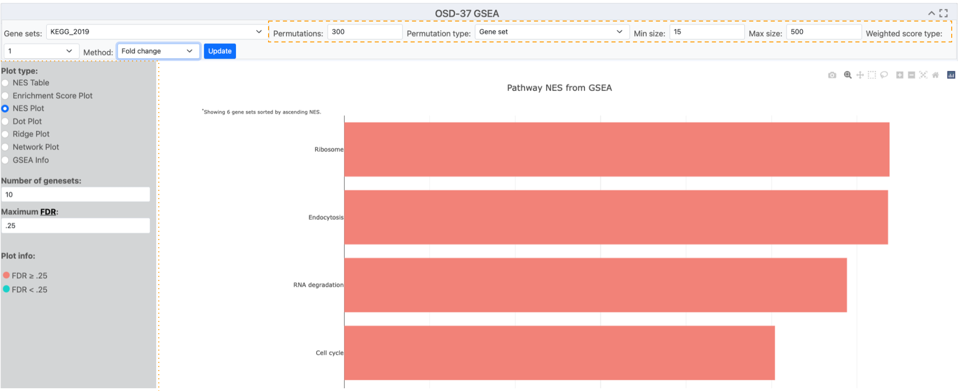
Image displaying a table of graphing options. The selection of options has created a red NES plot showing 4 terms (Ribosome, Endocytosis, RNA degradation and cell cycle) identified by GSEA analysis of the KEGG_2019 database. The permutation and gene list min and maximum parameters are highlighted with an orange dashed box. The plot-type menu has been highlighted with an orange dotted box.

Ontology databases and statistical methods used for analysis.

Selecting different databases for statistical analysis can identify different responses and provide alternative perspectives and insights from the results.

• Numerous ontology databases and statistical methodologies are available for application to the processed DESeq2 results.

  • Ontology database example description: A menu of pop-up menu databases can be opened, and one can be selected based on your model organism and question of choice. 5 different statical methods can be used by GSEA, signal to noise, T test, Fold change, Difference of class and Log2 Fold change.

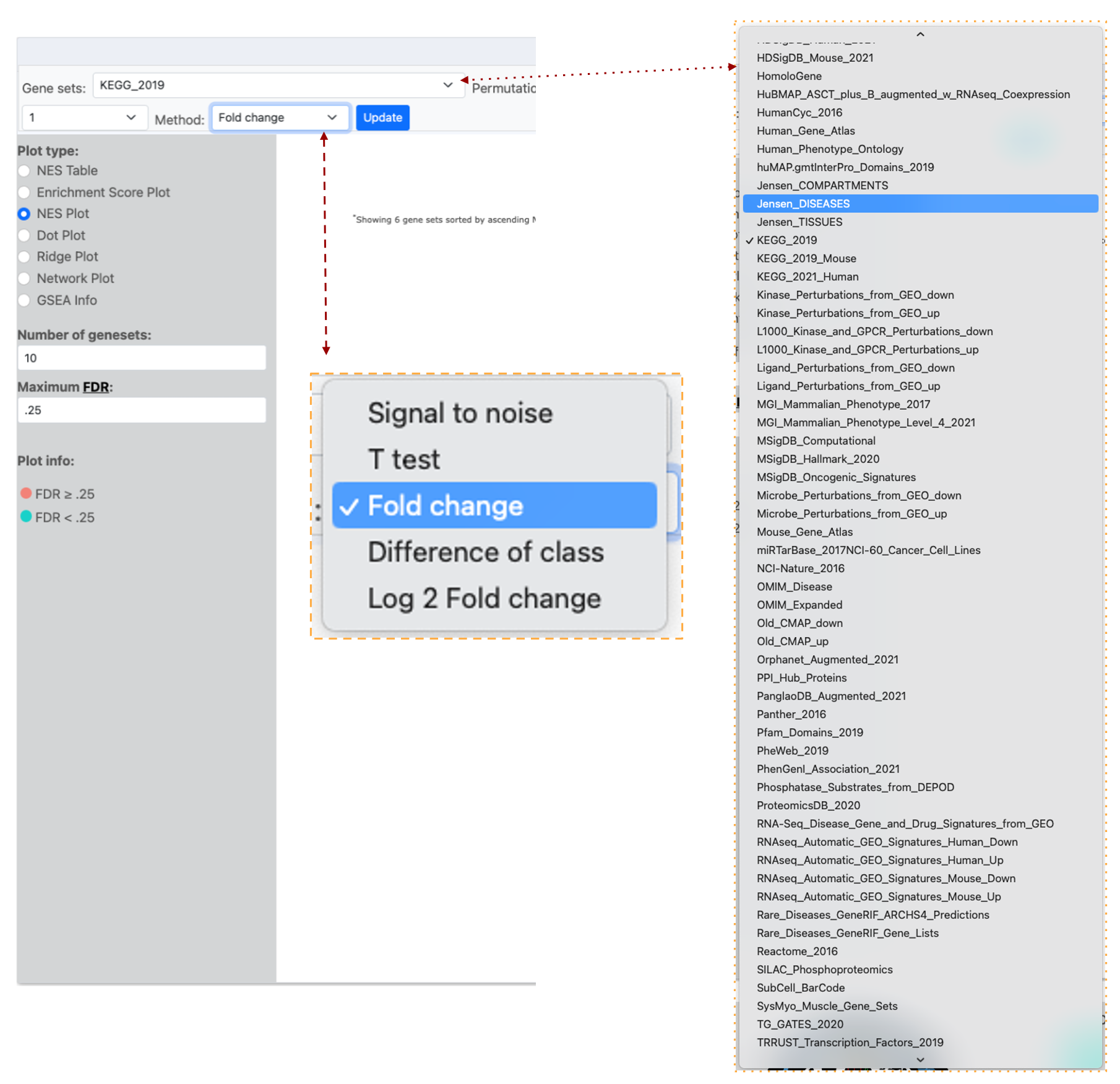
Image of half of the OSDR visualization page, the “Gene Set” menu has KEGG_2019 selected and a red dotted line links the list of accessible databases that can be selected from the connected drop-down menu that is highlighted by a yellow dotted line. The image also shows a red dashed line listing the different analysis “Methods” that can be used and the “Fold change” option is highlighted in blue to show it is selected.

Dot plots

Dot plots can present 3 types of data on the same graph.

The OSDR facilitates the visualization of the normalized enrichment score, false discovery rate, and Gene ratio values of all differentially expressed pathways on a single graph for user evaluation.

• Phenotype Permutation vs. Gene Set Permutation: Choosing the appropriate permutation method can influence your results. Phenotype permutation is generally preferred as it maintains the biological context of your experiment.

  • Example dot plot: demonstrating the analysis of the OSD-37 KEGG_2019 pathway employing the Fold change method and “Phenotype” permutation type. The Minimum and maximum size parameters were retained at their default values of 15 and 500 loci, respectively, as per standard practice. The quantities of “geneset”s” and the maximum false discovery rate (FDR) are set to their default values of 6 and 0.25, respectively.

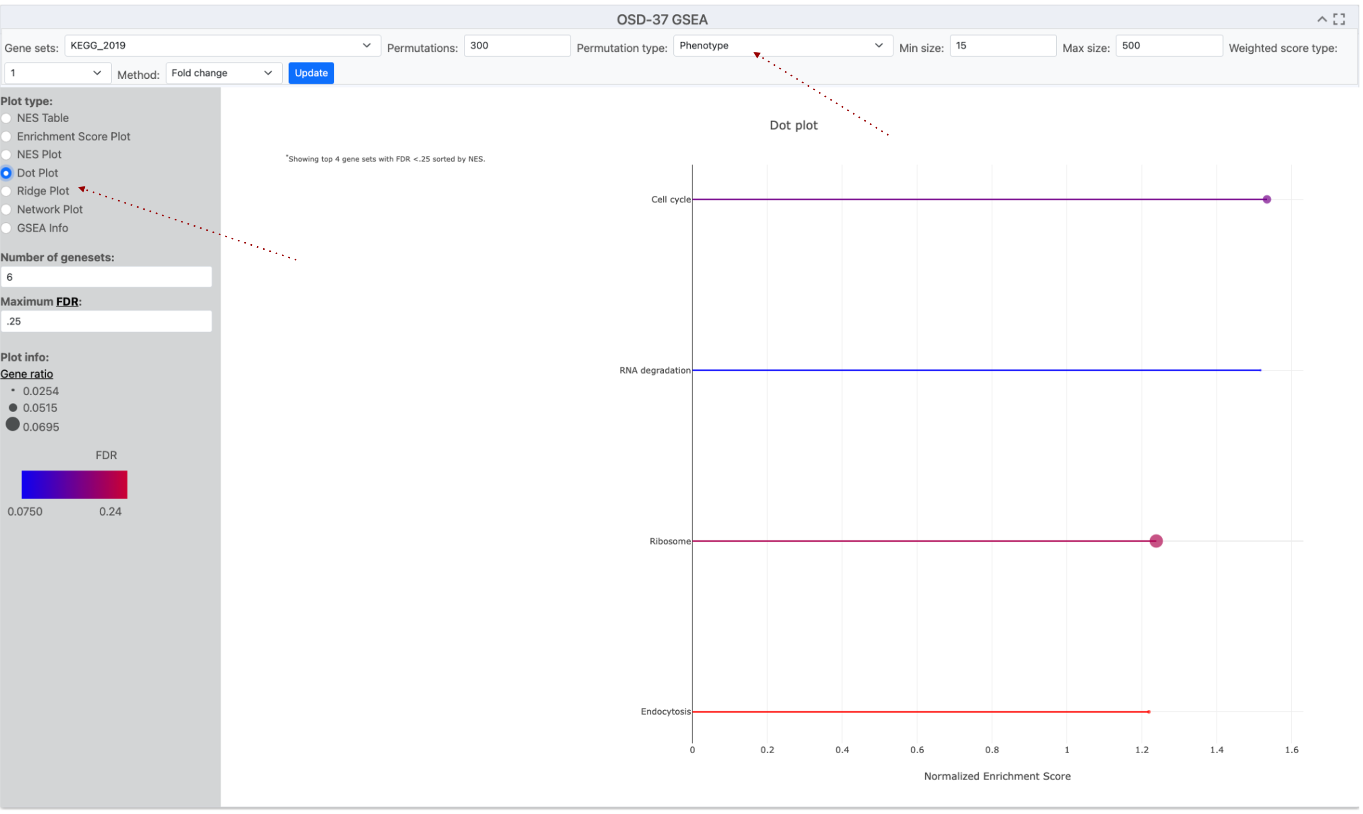
A screenshot of a Dotplot graph titled "OSD-37 GSEA." The x-axis label is "Normalized /enrichment Score" and the y-axis shows the name of the enriched KEGG pathway. The graph used two colors, red and blue to emphasize the variation in the FDR values for this data series. Data points size displays the Gene ratio value which is connected by lines to the pathway name on the Y-axis. Red dotted lines highlight where the Dot ploy options can be found and the “Phenotype” permutation has been selected.

Ridge plots

A ridge plot combines a density plot and a histogram to show how data, like Fold Change (FC), is distributed.

The OSDR facilitates the visualization of the false discovery rate (FDR), and Foldchange values of all differentially expressed pathways on a single graph for user evaluation. This visualization aids in determining whether genes are predominantly upregulated, downregulated, or exhibit minimal change. The smooth, ridge-like form reveals trends, and the plot is compatible with log-transformed data, a common feature in fold-change analysis. Overlaying plots for various groups allows researchers to compare fold-change distributions.

• Ridge plots are effective tools for present GSEA analysis.

  • Example Ridge plot: This example ridge-plot was made with a “Fold Change” of loci from the KEGG_2019 GSEA analysis data from OSD-37. The Minimum size and maximum size values were left to the default 15 and 500 loci as standard. The number of “geneset”s” and maximum false discovery rate (FDR) are set to their default values 6 and 0.25 respectively.

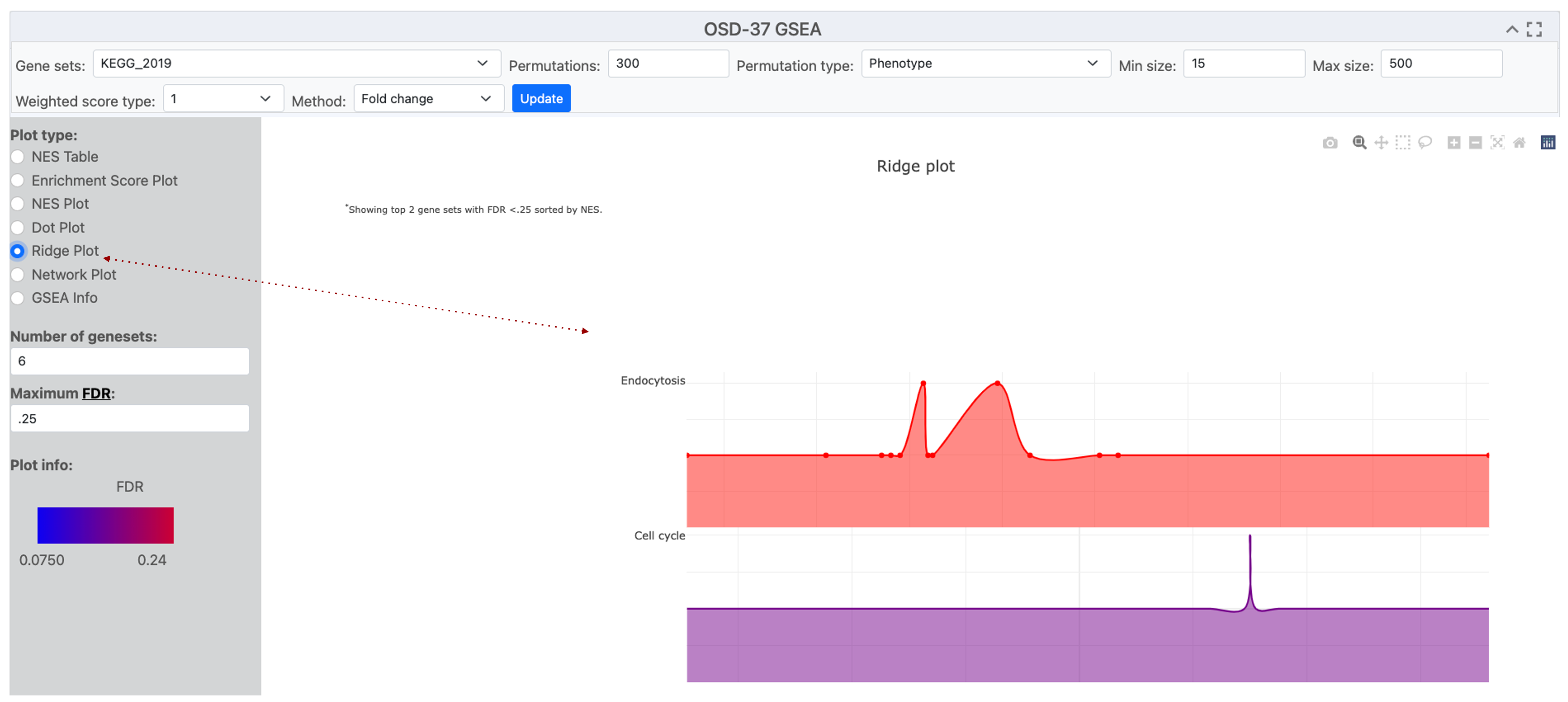
A screenshot of an Open Science Data Repository (OSDR) ridge plot page displays a ridge plot entitled "OSD-37 GSEA”. The Y-axis label shows the names of the terms detected by enrichment analysis of the selected gene sets eg Endocytosis and Cell cycle. The x-axis label is "Gene Fold Change”. Red dotted line highlights where the “Ridge Plot" option was engaged.

Network Plot

A network plot uses dots that represent nodes of data points that describe the response detected in the analysis.

• Network plots are effective tools for showing the variation in the number of genes involved in a detected response.

  • Example network diagram: it can be observed that the Ribosome possesses a greater number of loci that were implicated in that response ontology group. Even though “RNA degradation” and “Cell cycle” demonstrate a lesser quantity of associated genes, it is evident that they possess heightened significance due to their diminished adjusted P-value, as delineated by the gradient ranging from blue to red.

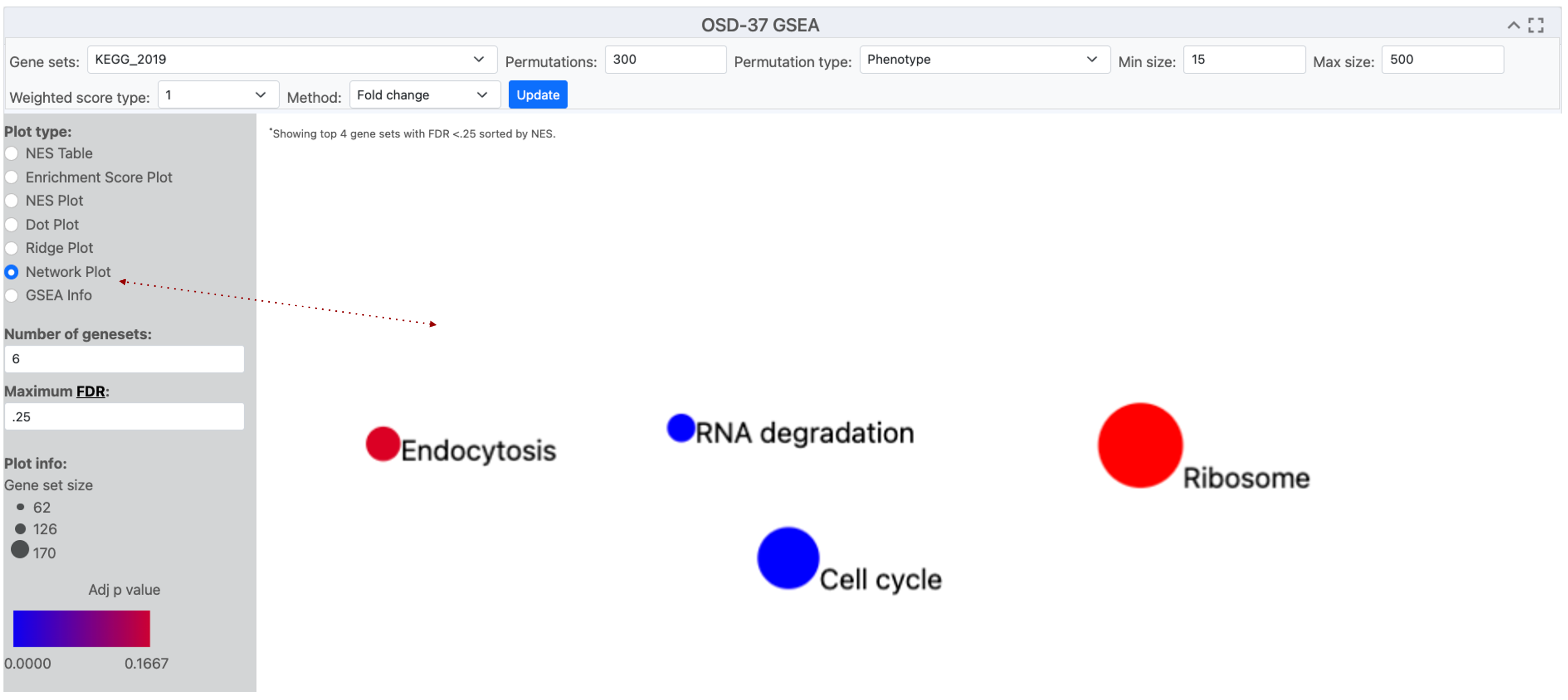
A screenshot of an Open Science Data Repository (OSDR) network plot page with the title OSD-37 GSEA. In the center a plot shows 4 circles, representing enriched terms from the KEGG_2019 database. The size of the dots indicates the number of genes detected in that GO group and the red-to-blue color gradient shows the significance of their enrichment. A red dotted line highlights where the network plot was selected

Network Plot used in conjunction with pathway illustration

A network plot uses dots that represent nodes of data points that describe the response detected in the analysis.

• Network plots can be merged with pathway diagrams to help illustrate connections between enriched terms and concepts like cellular function. Figures can then be shared with other OSDR AWG collaborators on platforms like GitHub as staging for eventual publication in Zenodo and peer-reviewed journals.

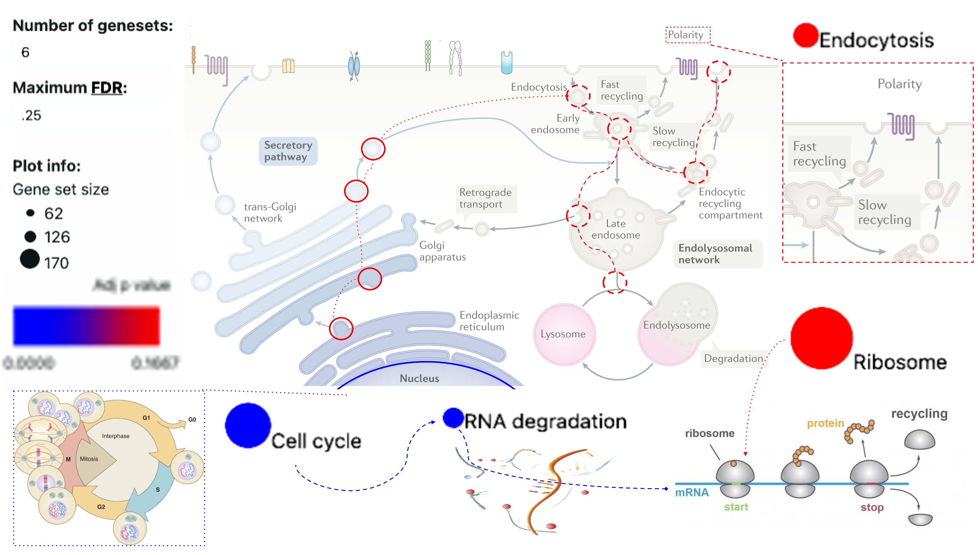
The previous network dots and plot information have been incorporated into the endocytosis diagram to illustrate how these KEGG pathway terms related to cellular biology. The use of pop-out boxes and dotted or dashed lines is used to show connections based on knowledge from the literature.

NES plots

NES (Normalized Enrichment Score) plot offers a visual representation of the normalized enrichment score for gene sets identified by the user based on their parameters.

• NES plots are an effect tool for viewing pathways that are identified by GSEA.

  • Example NES plot: The data from OSD-37 provides the normalized enrichment score adjacent to terms that possess enrichment in the selected database. KEGG_2019 was used as the “geneset” for enrichment analysis. However, in this instance, we show that it is possible to change the analyzed database. The bar plot then displays GO terms identified during the analysis when the GO_cellular_Componet_AutoRIF gene set database was queried.

This image shows a NES plot and the options used to generate it. Situated at the top of the webpage is a search bar that facilitates the exploration of specific terms within the datasets and other “geneset" for analysis. Immediately beneath the search mechanism is a tabular structure providing alternative plot types and graph parameters. The bar plot structure summarizes distinct gene groups that are known to function in a similar location based on the GO-Cellular_Component_AutoRIF enrichment analysis. The Red dotted lines highlight the “number of “geneset”s” and the method values have been adjusted from their default values.

Enhancing NES plots

Adjusting the parameters to influence the quantity and sequence of pathways detected.

• NES plots have a numerical constant that can be adjusted to modify the appearance pathways that GSEA identifies

  • Numerical method example: In this OSD-37 example we’ve changed the “Method” value to 0 (classic), which changes the normalized enrichment score and graph layout.

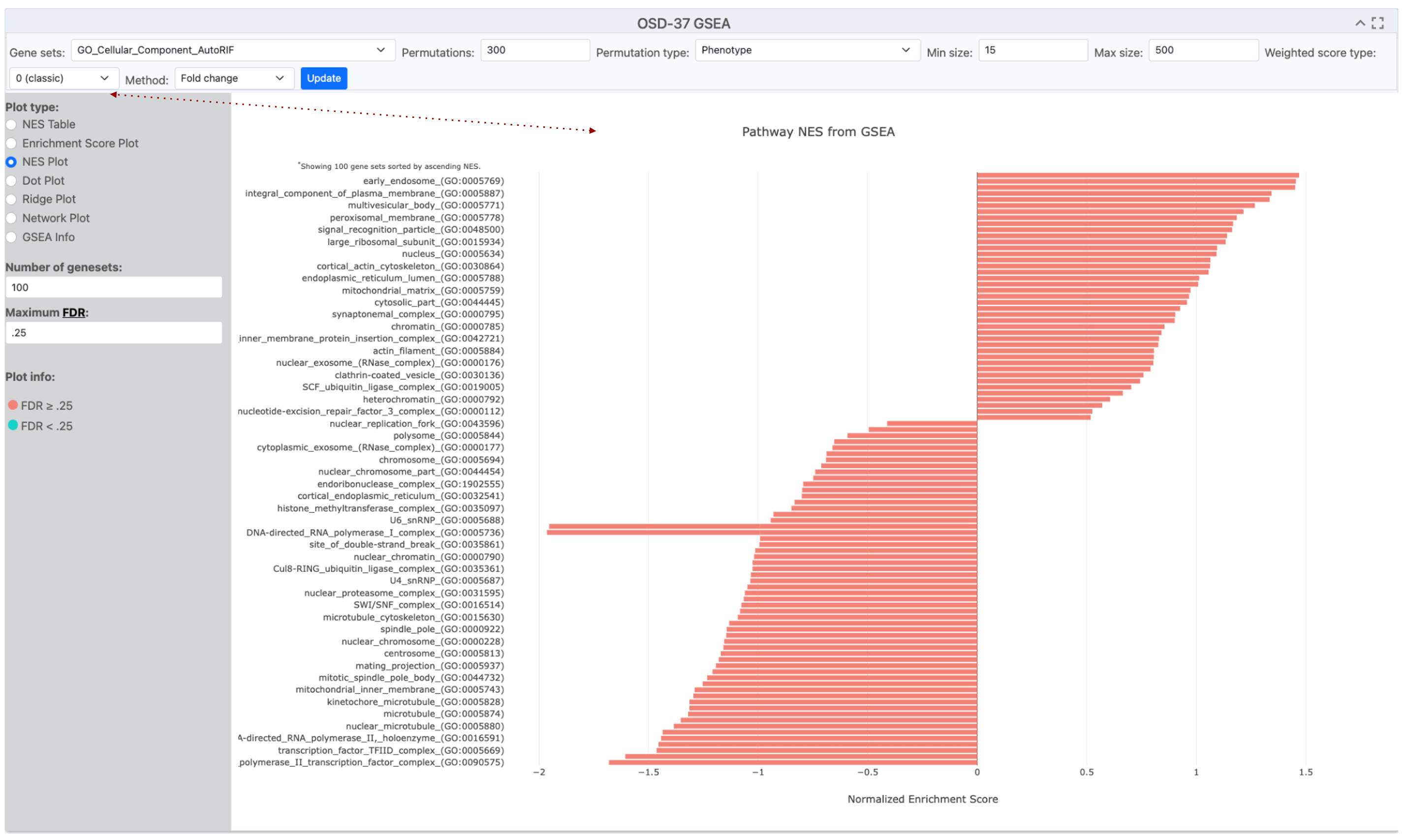
This image shows a NES plot and the options used to generate it. The bar plot structure summarizes distinct gene groups that are known to function in a similar location based on the GO-Cellular_Component_AutoRF enrichment analysis. The red dotted line highlights that the “Method” is currently set to 0 (classic mode) but was set to 1 in the previous figure.

Refining NES plots using the Method Value

Adjusting the “geneset” is highly recommended in the Method tab and can change the number and order of pathways identified.

• When utilizing a normalized enrichment score plot (NES plot) to depict pathway enrichment via the fold change method, the graphical representation not only illustrates pathways with statistical significance but incorporates pathways that lack such significance.

  • Number of “genesets” example: In this example, the “Method” value is set to 1, and we’ve changed the “geneset” to Cellular_Component_AutoRIF_Predicted_zscore. Notice that the number of “genesets” is now set to 15 and that the color coding shows that only 4 of these are significant based on the current threshold of a maximum False Discovery Rate of 0.25.

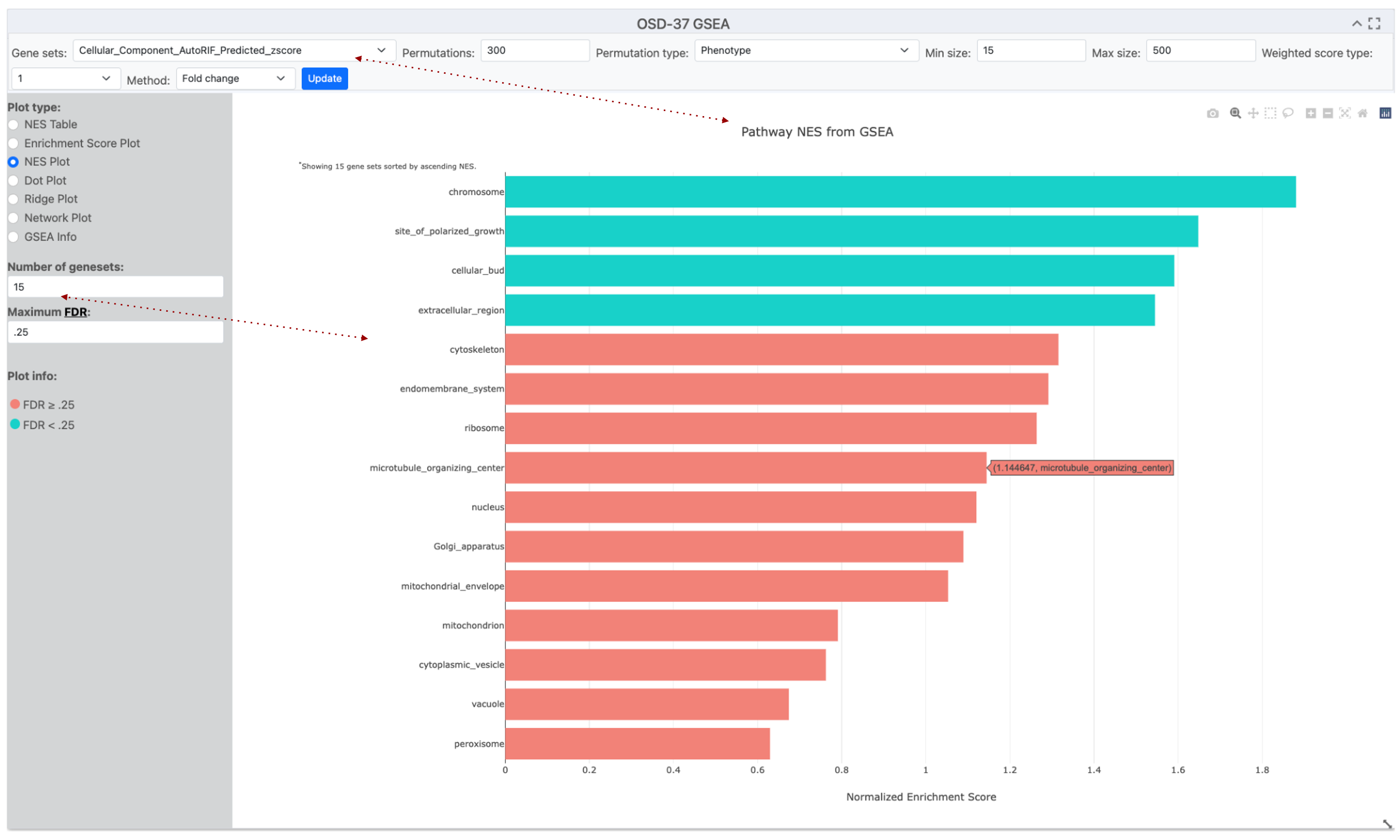
This image displays a screenshot of the OSDR Visualization software, which includes an NES plot graph and the parameters used to create it. The NES bar plot structure summarizes distinct gene groups known to function in a similar cellular location based on GO-Cellular_Component_AutoRIF_zscore enrichment analysis. The method is currently set to 0 1, and the number of “geneset”s included was set to 15, with coloring determined by a 0.25 False Discovery Rate (FDR) cutoff threshold. Red arrows highlight the Gene sets and number of “geneset”s selected for this enrichment analysis.

Fine-tuning permutations

Adjusting the permutation value can be used to improve the GSEA statistical model.

GSEA calculates enrichment scores by comparing the data to a random null distribution. This null distribution is generated by permuting the phenotype labels of your samples numerous times. A higher number of permutations leads to a more precise estimation of the p-value associated with your enrichment score.

• You can choose the number of permutations to run, with a higher number leading to potentially more accurate p-values.

  • Example Finetuning Permutations: Altering the default premonition from 300 to 500 in the example description resulted in a significant change in the FDR of the “cytoskeleton” Gene Ontology term.

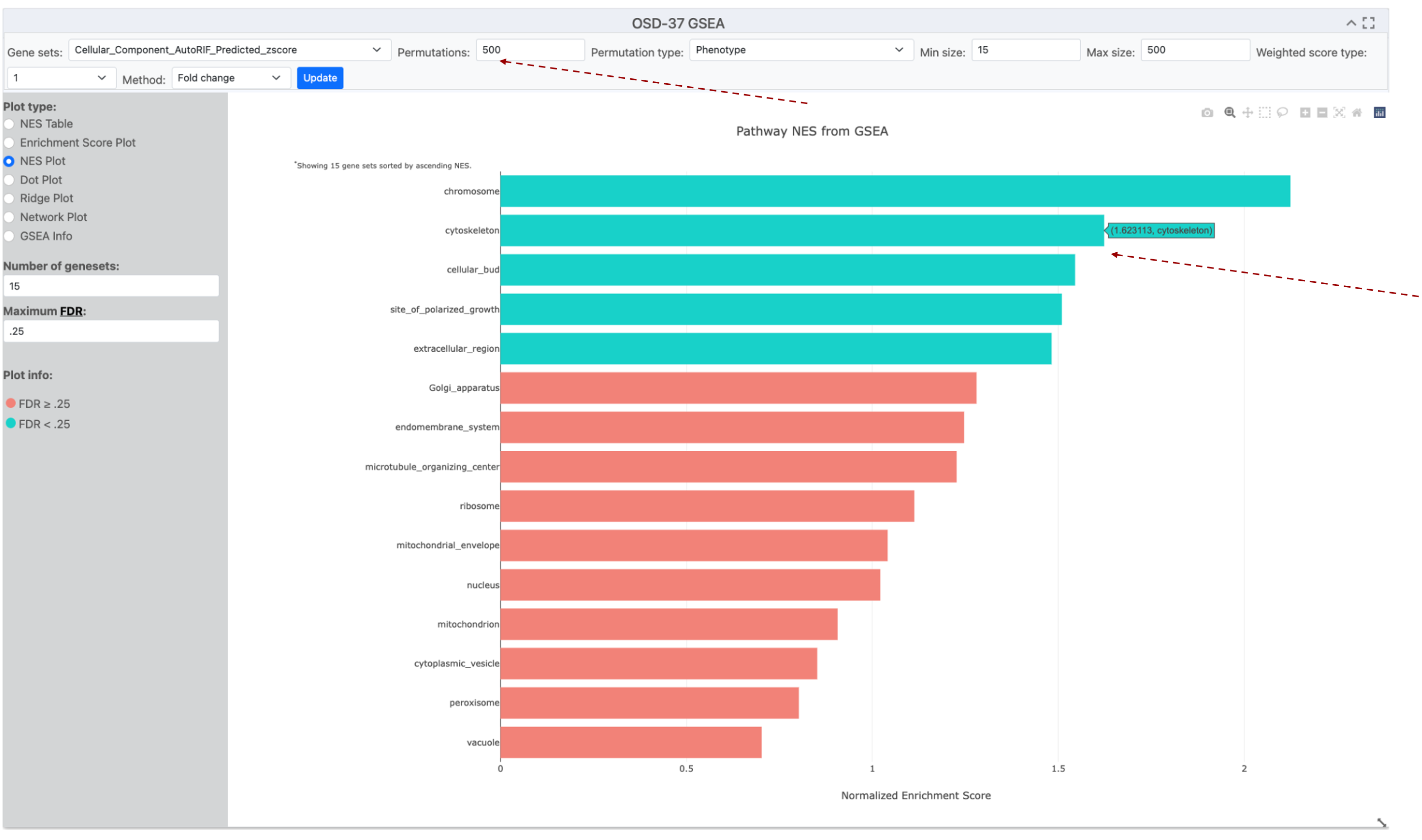
This image displays NES plot graph and the parameters used to create it. The NES bar plot structure summarizes distinct gene groups known to function in a similar cellular location based on GO-Cellular_Component_AutoRIF_zscore enrichment analysis. The method is currently set to 1, and the number of “genesets” included was set to 15, with coloring determined by a 0.25 False Discovery Rate (FDR) cutoff threshold. The permutations number has been increased to 500 and the cytoskeleton GO term has increased its NES score and changed from the Red FDR>0.25 to the Blue FDR<0.25 group. Red arrows highlight the permutation value has been increased and that moving the mouse over a bar creates a popup that provides its name and value.