Results

We flew plants on a rocket — then measured what changed

A real MadWest dataset. It starts with the stimulus — a payload carried aloft on a sounding rocket — and follows it into two readouts of what the flight did: gene expression (the Reggies' Veggies qPCR arm, below) and seedling growth (the TREES timelapse, by image analysis). Everything is packaged for NASA OSDR.

Four launches, one program

The results below come from a program of four sounding-rocket launches (2018–2019). "Reggies' Veggies" and "TREES" are two of the 2018 launches — TREES is a launch codename, not a species. The 2019 mission, Project Ariadne, flew slime mould.

🌱

Launch 1 · Arabidopsis test

Flown seedlings showed earlier flowering, and co-flown ectomycorrhizal spores stayed viable after the flight.

🧬

Launch 2 · Arabidopsis (qPCR)

The repeat that produced the Reggies' Veggies gene-expression samples analysed just below.

🌳

Launch 3 · TREES

Populus tremula (aspen) × ectomycorrhiza — the survival timelapse further down.

🧠

Launch 4 · Project Ariadne (2019)

Physarum polycephalum slime mould — flown to test hypergravity-induced behavioural changes, then placed in 3D-printed mazes post-recovery. See the Ariadne page →

Launch 2 · gene-expression arm

The molecular arm — Reggies' Veggies

It begins with a flight. In the Reggies' Veggies experiment (launch 2), Arabidopsis was flown on a sounding rocket alongside launch-site and lab controls, then assayed by qPCR for stress-response genes — asking what the flight changed inside the plants. Its companion, the TREES survival timelapse further down (launch 3), asks whether a fungal partner could help a tree survive the flight. Together they pair a gene-expression readout with a growth phenotype — exactly the kind of multi-measurement story OSDR is built to hold.

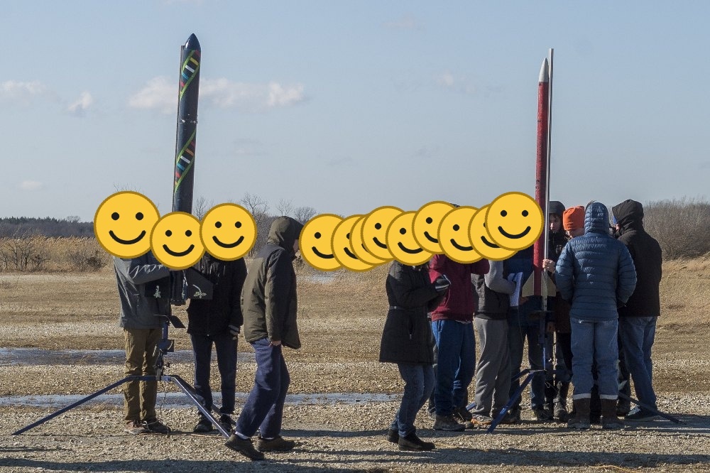
The rocket on the launch rail with the student team

Launch day — the payload heads up on a K1620 motor.

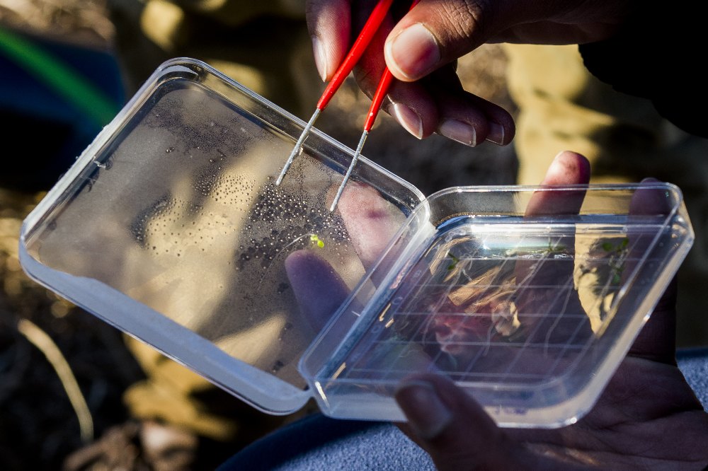
Pipetting seedling samples on agar plates in the lab

Back in the lab — preparing samples for RNA extraction.

Flight profile

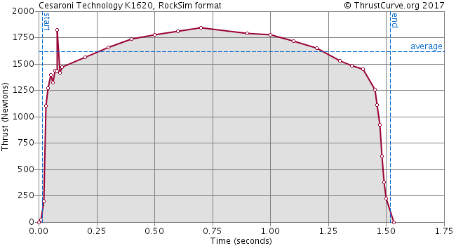
The payload flew on a K1620 motor, with onboard altimeters logging the flight. The motor's thrust curve and the raw altimeter exports are included in the data deposit as the environmental context for the biology.

Genes assayed (qPCR)

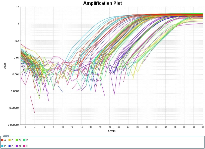
Expression of plant stress-response genes was measured by qPCR, normalized to a housekeeping reference. Amplification plots and raw runs are in the deposit.

Gene	Role in the plant
UBQ10	Reference / housekeeping (normalizer)
MPK3	Stress-signaling MAP kinase
TCH3	Touch / mechanostimulus-induced
CBP / CBP60g	Calmodulin-binding; defense signaling

What the genes did — ΔΔCt fold-change

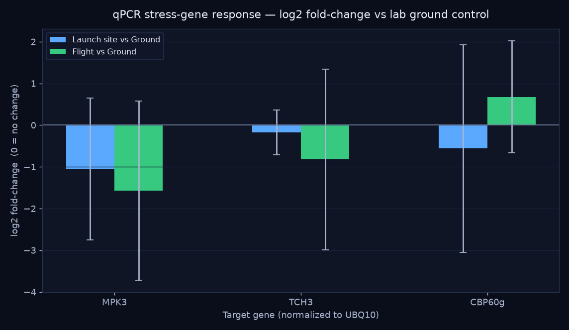
Per-well Ct values from the qPCR exports were normalized to the UBQ10 reference gene and expressed as fold-change relative to the lab ground control (the standard ΔΔCt method). Four biological replicates per group.

qPCR log2 fold-change of stress genes by treatment

Gene	Launch site	Flight
MPK3	0.48×	0.34× ↓
TCH3	0.89×	0.56× ↓
CBP60g	0.68×	1.60× ↑

Flown plants trended toward lower MPK3 and TCH3 (stress- and touch-signaling) but higher CBP60g (defense signaling) versus the lab control — a hint that flight shifts which stress pathways are engaged rather than simply turning "stress" up or down.

Read as a trend, not a result. With n = 4 and wide biological spread, the error bars cross "no change" for every gene — none of these would survive a significance test as-is. They're a genuine, reproducible ΔΔCt computation on real data, valuable as a method demonstration and a hypothesis to test with more replicates. (One grouping caveat: sample IDs 22/23 are labeled differently between the plate design and the tube log — see DEVLOG.md.)

Launch 3 · the survival experiment

TREES — can a fungal partner help a tree survive flight?

TREES is the third launch's codename. Its host was the aspen Populus tremula, and the "microbe" was an ectomycorrhizal (ECM) fungus — a root symbiont. The hypothesis: the tree–fungus symbiosis would help the seedlings survive the rigors of flight. Seedlings grew on gridded agar plates and were imaged as a timelapse under a 2×2 design crossing ECM inoculation with rocket flight — 13 plants, ~2,600 frames, up to ~12 days.

	+ ECM (mycorrhizal)	− ECM
Flight (rocket)	MR · +ECM · Flight (4 plants)	R · −ECM · Flight (2 plants)
Ground control	M · +ECM · Ground (5 plants)	X · −ECM · Ground (2 plants)

The ECM fungal species isn't recorded in the surviving lab files, so it's noted as unknown in the data package. add species if known

All four treatments, side by side

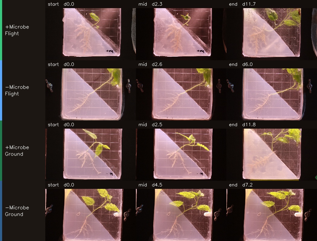
Each plant plays through its own timeline so you can compare how the groups developed. Watch the +ECM (mycorrhizal) plates especially — several green up, then brown and collapse. The day counter in each tile is elapsed time for that plant.

What the image analysis found — the symbiosis didn't rescue them

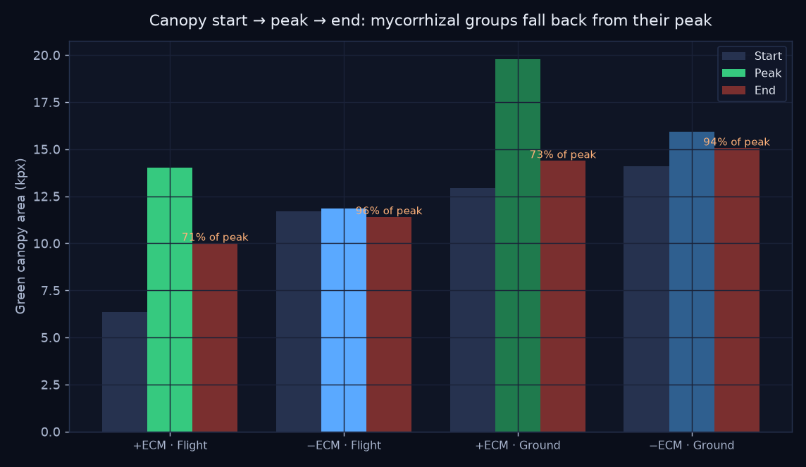
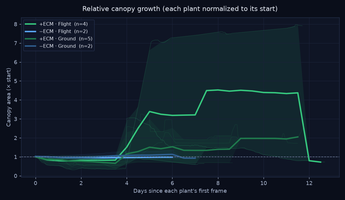
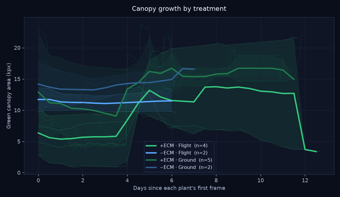
Tracking green-canopy area frame by frame tells a story a single snapshot misses: the mycorrhizal (+ECM) seedlings peaked, then declined — ending at only ~71–73% of their peak canopy, with several collapsing far further (one flown +ECM plant fell to 22% of its peak). The non-mycorrhizal plants held near their peak (94–96%). Contrary to the hypothesis, the fungal partner did not help the trees survive — the +ECM groups slowly died back across the timelapse.

Start, peak and end canopy per treatment showing mycorrhizal die-back

Read with care — the windows differ

Classroom-scale (2–5 plants per group). Crucially, the +ECM groups were imaged ~9 days but the −ECM groups only ~6 — so the −ECM plants may simply not have been watched long enough to meet the same fate. The mycorrhizal die-back is real and visible in the footage, but this is a strong trend, not a controlled proof. The other contribution is the method: turning plate photos into quantitative, OSDR-ready growth trajectories.

Orange labels show end canopy as a percentage of each group's peak — the shortfall is the die-back.

Relative canopy growth curves by treatment

Each plant normalized to its own starting canopy. Thick line = treatment mean; faint lines = individual plants; band = min–max spread.

Absolute canopy growth curves by treatment

Absolute green-canopy area (kilo-pixels at a fixed analysis width). Same plotting convention as the relative chart.

Individual timelapses

One representative plant per treatment, full resolution.

+ECM · Flight — plant mr1-1

−ECM · Flight — plant R3-3

+ECM · Ground — plant m2-3

−ECM · Ground — plant X4-1

How the analysis works

🟢

1 · Segment

Each frame is reduced to its green canopy using the Excess-Green vegetation index, with near-white backlight glare removed. Roots and the frosted cover are excluded.

📈

2 · Quantify

Canopy area (in pixels at a fixed width) is logged per frame with its timestamp, then smoothed and normalized per plant to control for plate-to-plate scale.

🧮

3 · Compare

Plants are averaged within each treatment on a common time grid, producing the growth curves and the start → peak → end comparison that reveals the die-back.

The full pipeline lives in analysis/ (segment_lib.py, analyze.py, make_timelapse.py) and writes a tidy growth_data.csv — one row per frame, ready to reshape for an OSDR submission.