- description: >-
The OSDR RadLab application is a valuable tool for researchers and scientists
who need access to radiation measurements from space.
RadLab Overview
Please follow this link to access the **RadLab OSDR Visualization application**.
The application provides a central repository for radiation data from a wide variety of sensors that have flown on various spacecraft. This makes it easy for users to find and access the data they need, regardless of the specific sensor or spacecraft that collected it.
The OSDR RadLab application is also a powerful tool for data analysis. It provides a variety of features that allow users to visualize, analyze, and compare radiation data. This can be helpful for identifying trends and patterns in the data, as well as for understanding the effects of radiation on different materials and systems.
One of the most important features of the OSDR RadLab application is its ability to connect primary radiation data with metadata such as vehicle and time. This information is essential for understanding the context in which the radiation data was collected. It can also be used to filter and sort the data, making it easier to find the specific information that users are looking for.
The OSDR RadLab application is a valuable resource for researchers and scientists who need access to radiation measurements from space. It is a powerful tool for data analysis and visualization, and it can help users to understand the effects of radiation on different materials and systems.
Data overview page
When you first land on the RadLab you start in the “data overview” page.
This page summarizes the different sensors, the time they were collecting data and the space vehical they were on. The graph is interactive so the users can select subsets within the data to drill down and the graph will rearrange to optimize the data visualization. On the bar on the left the user can then navigate down to a range of different visualization options.
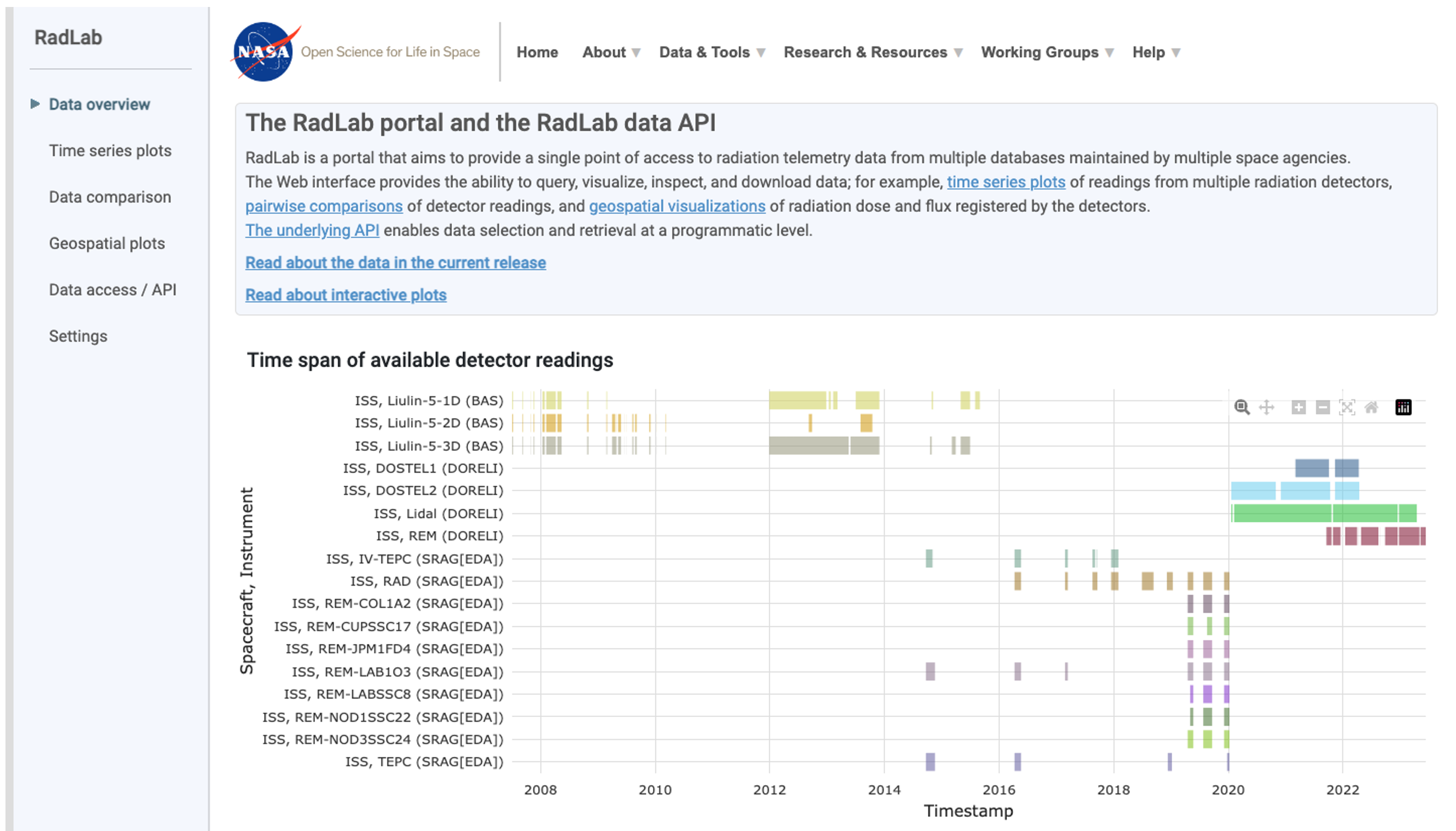
Screenshot of a data overview webpage titled “RadLab portal and the RadLab data API” on the NASA website. The page shows a time graph of available detector readings. The y-axis shows the number of detectors and the x-axis shows the timespan.
RadLab Time series line plots
When you first land on the Time series plot page the graphs initially appear empty
This page allows users to view the radiation data but requires users needs to define the periods and sensors of interest.
In this example, a Red arrow highlights how users can quickly load a preselected period to help get familiarized with the interface.
Select either “Total dose rate” or “Total flux” values.
The user can alternate between a “Linear” and “Log” scale.
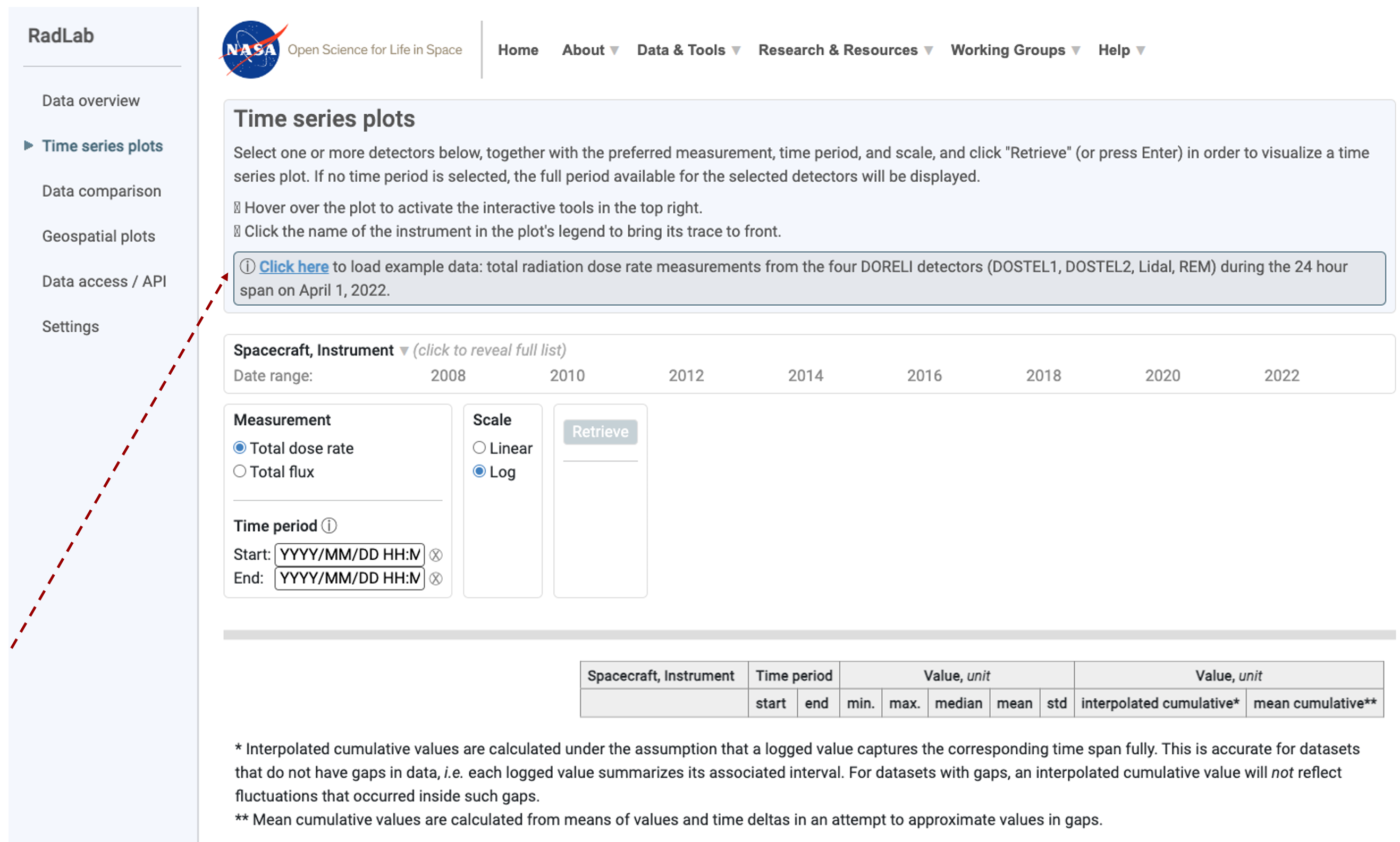
Screenshot of a data overview webpage titled “Time series plots” on the NASA RadLab website. On the initial landing page doesn't contain any data, the red arrow highlights the “click here” button that loads an example data set. There is an empty template that shows time on the x-axis and provides the user with the chance to load different spacecraft, instruments or specific time period.
Selecting periods for closer inspection
In this example 4 sensors have been selected for a 2-day period, an orange box highlights how a user can click on the graph and make a selection lasso to define a smaller region such as a 5-hour period as highlighted by the red arrow. The user can then explore the graph using the mouse to reveal metadata about the spacecraft, instrument, data source, time stamp, and total dose rate.
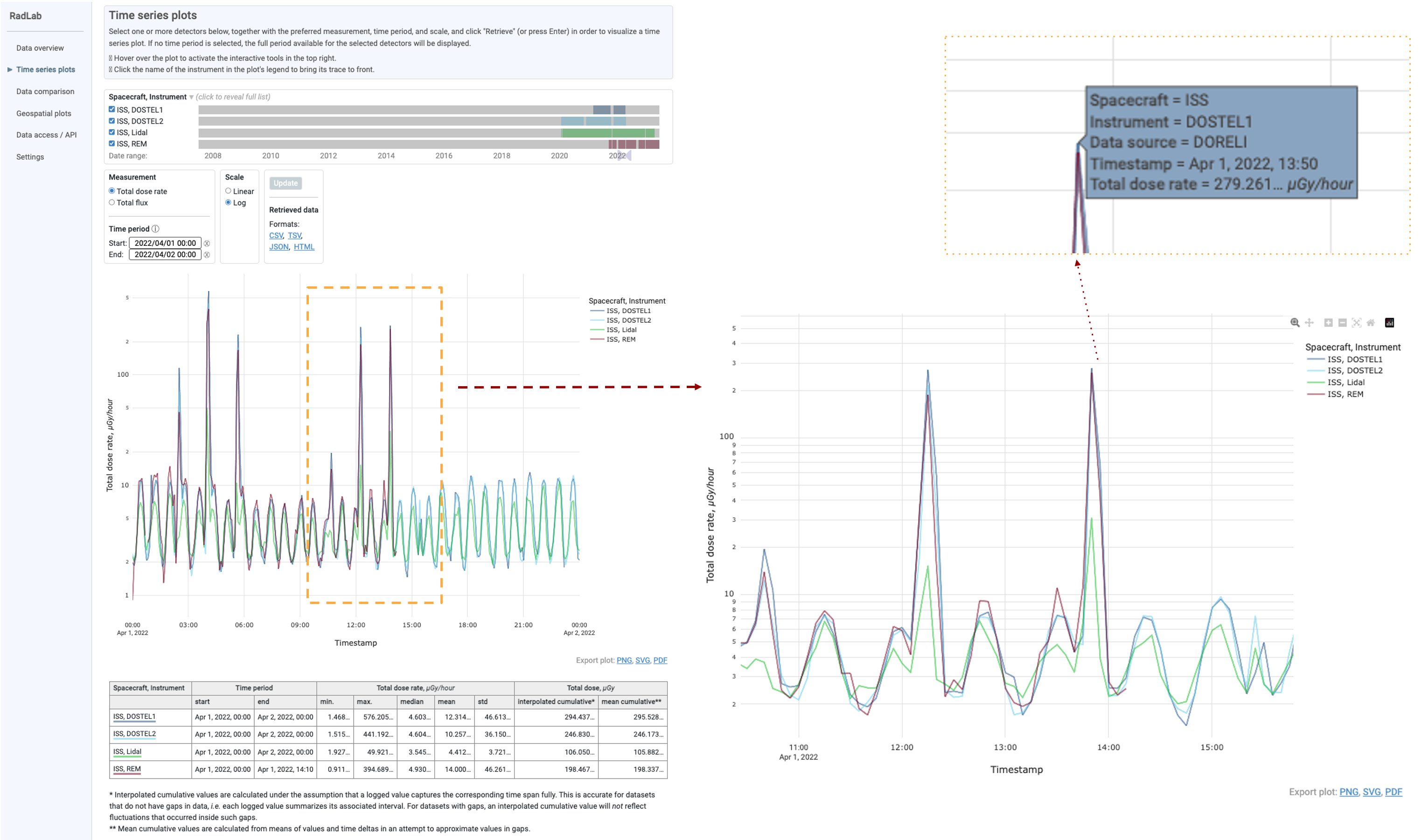
Screenshot of a “Time series plots” on the NASA RadLab website. On the initial landing page, an orange box highlights periods that were selected by clicking on the screen. To the right is the zoomed-in view that shows these data with greater resolution. The orange dotted box shows that when the user moves the mouse over the graph additional data is shown. Time on the x-axis currently shows 3 different types of sensors on the ISS.
Data comparison
In this example, the user has selected a specific point in time and have decided to use regression to compare the results from 2 different types of sensors. The images show the meta options that were used to compare the REM and Lidal sensors. The orange dashed lines show how the user has selected. Region of the graph, this then updates allowing the user to see the data at a high resolution. The 3rd inserts zoom in to show that these graphs are interactive allowing the user to highlight specific data points using their mouse to acquire further information as to how that data point was acquired.
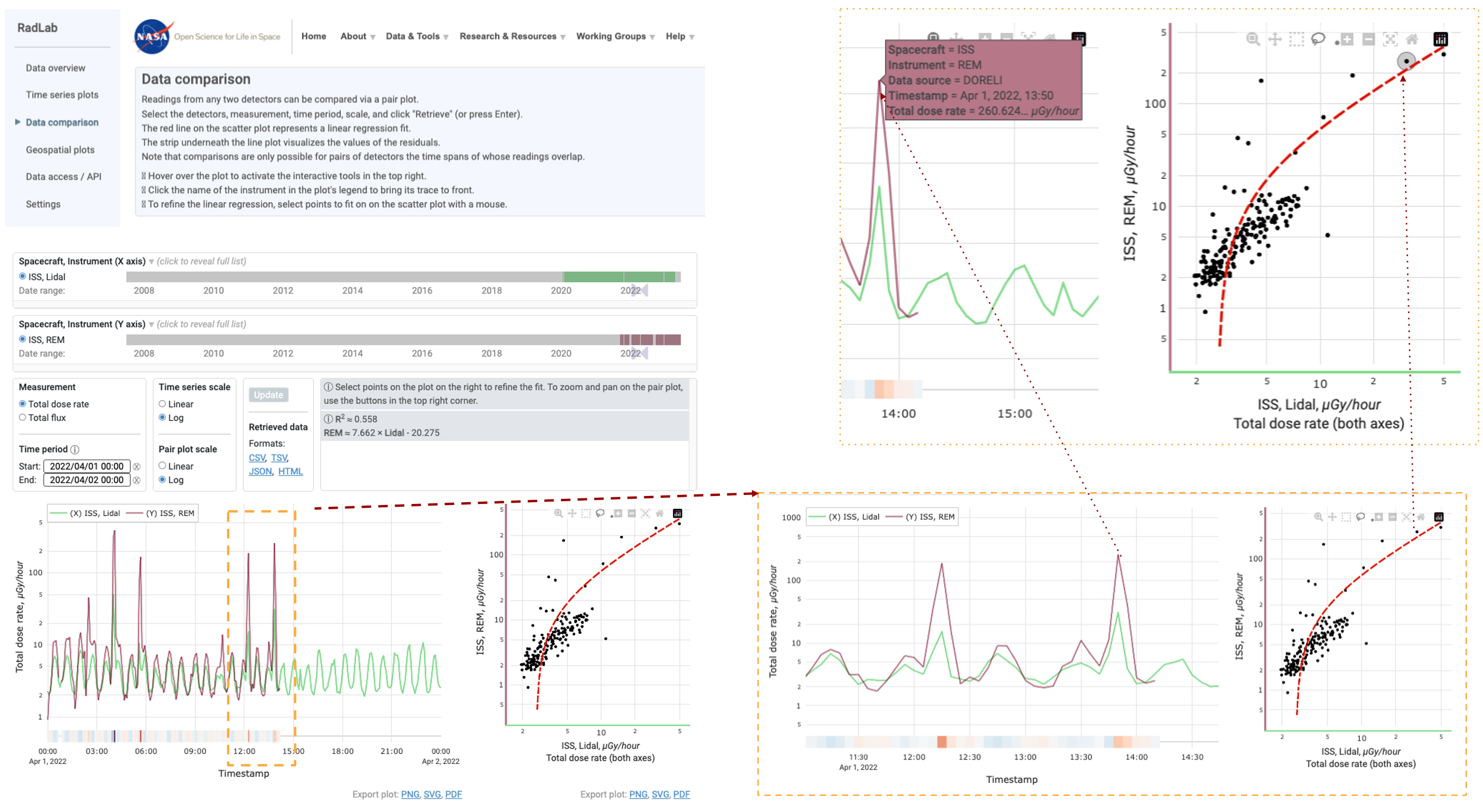
Screenshot of a “Data comparison” on the NASA RadLab website. On the initial landing page, an orange box highlights the periods selected by clicking on the screen. To the right is the zoomed-in view that shows these data with greater resolution and allows the user to linear regression comparing different combinations of sensors. The orange dotted box shows that when the user moves the mouse over the graph additional data is shown. Time on the x-axis and currently shows 3 different types of sensors on the ISS.
Geospatial plots
When the Geospatial plots page loads it starts empty.
In the example below we’ve highlighted that there is a demo option that loads data from the lidal detector for the year of 2022.
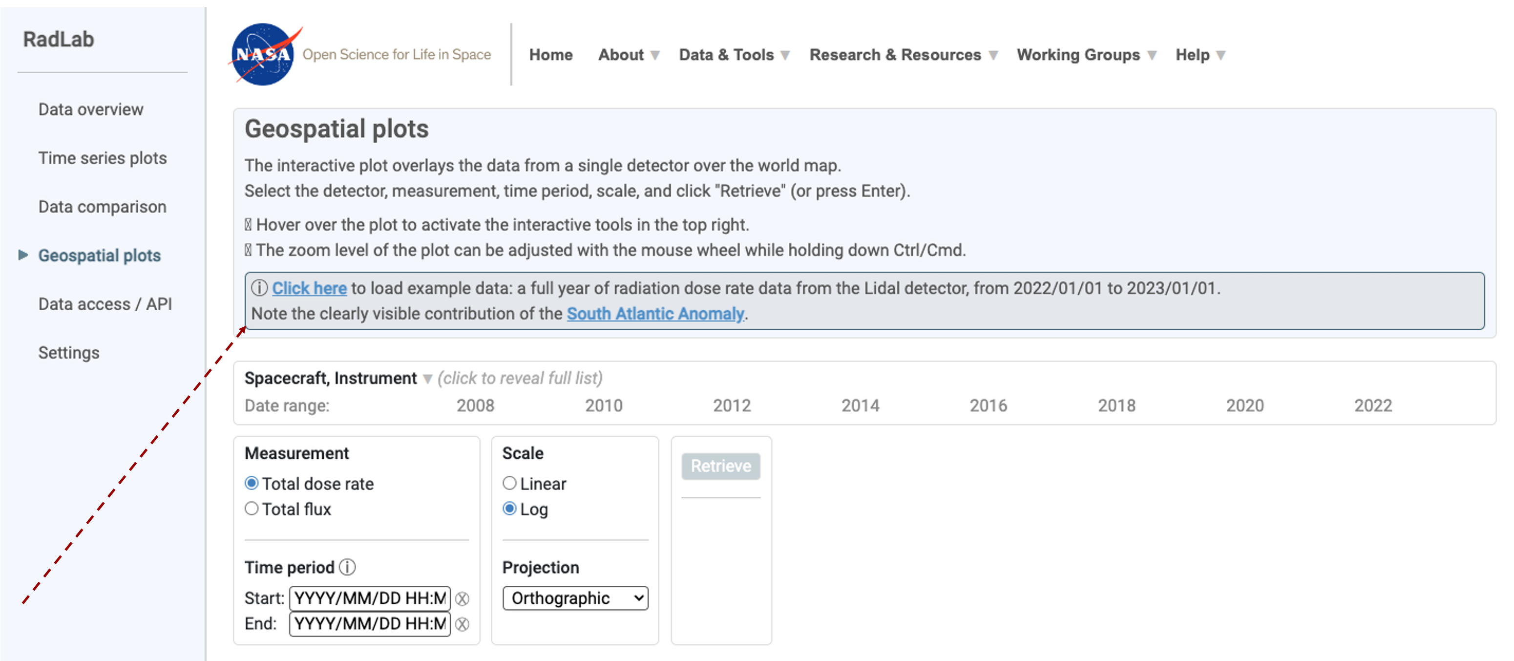
Screenshot of a data overview webpage titled “Geospatial plots” on the NASA RadLab website. On the initial landing page, a red arrow highlights the “click here” button that loads an example dataset. There is an empty template that shows time on the x-axis and provides the user with the chance to load different spacecraft, instruments, or specific time period.
Geospatial orthographic projection
The geospace plot page contains information about the spacecraft, the time period, the instrument, the measurement type, the scale of data transformation, the current projection type being used and also allows the users to down the data as a .csv, .txt, .json, and/or .HTML.
In this example the demo data from 2022 has been loaded, the log scale selected, allowing us to the Total dose rate as measured by the Lidal sensor.
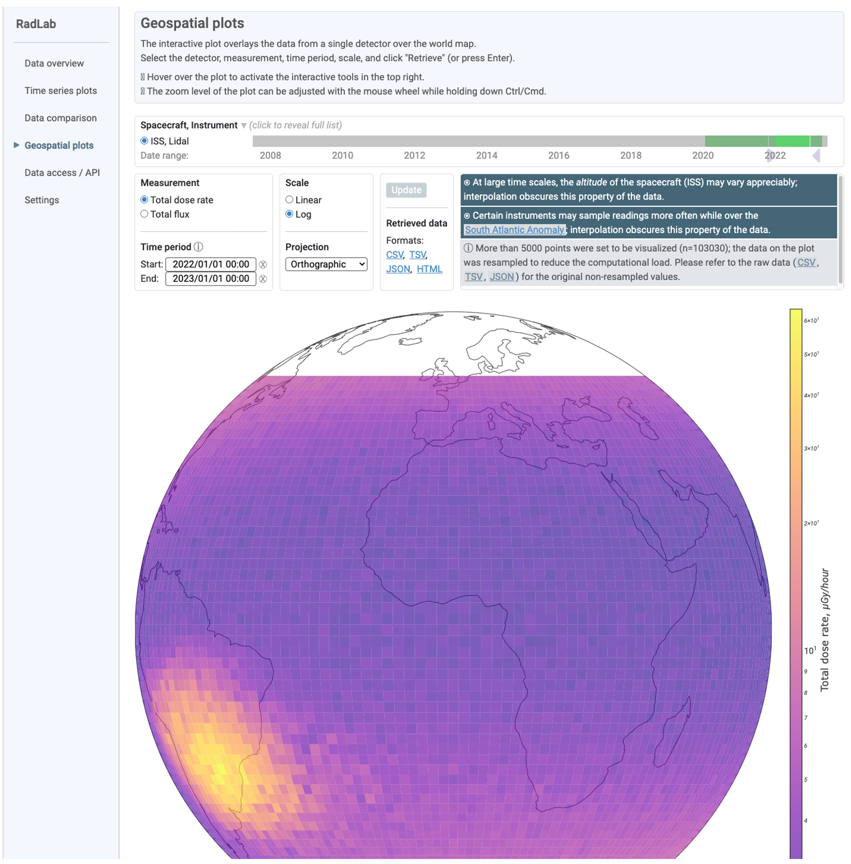
Screenshot of a Geospatial data overview webpage on the NASA RadLab website where the example dataset has been added, it shows data from an ISS Lidal sensor from a period of 2020-2022 as an orthographic projection. The data is then plotted on the map showing a radiation hot spot above the South Atlantic Ocean.
Other Geospatial options
The RadLab allows users to change the type of geographical pot they use to present the data. In this example, we can see a comparison of 2 different methods, the equal Earth and natural earth. We recommend you explore them all and choose the one that is best for you.
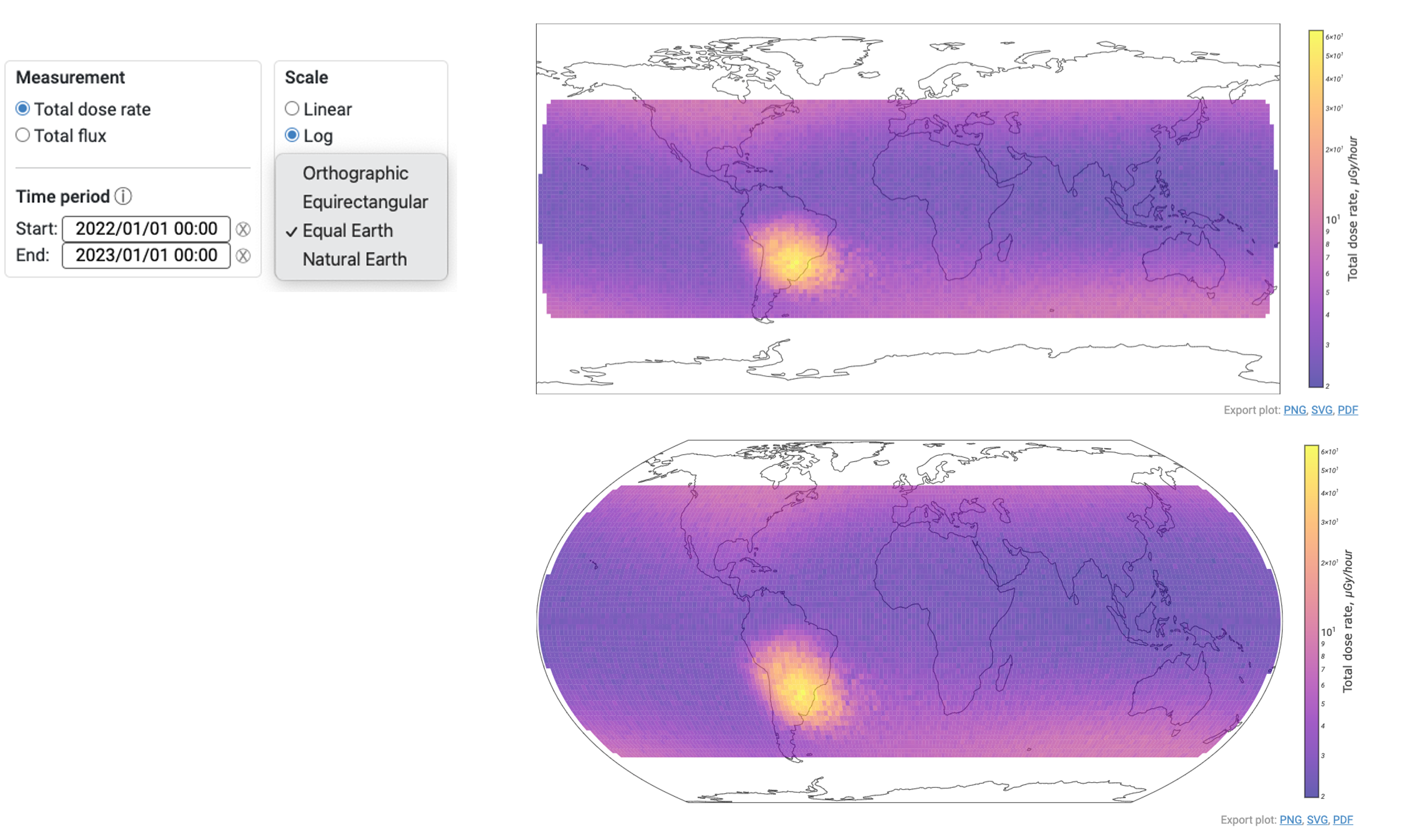
Screenshot of a data overview of 2 different ways to project the data with an insert showing the options that currently include Orthographic, Equirectangular, Equal Earth, and Natural Earth. The example dataset has been added, it shows data from an ISS Lidal sensor from the period of 2020-2022. The data is then plotted on the map showing a radiation hot spot above the South Atlantic Ocean.
RadLab sensor color definitions
This page provides a list of all instruments in RadLab, along with the data source, the spacecraft, and the color that RadLab uses to define them through the analysis. This page also reminds users to clear their “cookies” is they have previously saved any settings.
.png)
Screenshot of a NASA RadLab website “Settings” page, it lists all the instruments that are currently in the RadLab database. The data is then plotted on the map showing a radiation hot spot above the South Atlantic Ocean.